Basics of texture mapping

Early on, rasterizers only dealt with generating procedural detail across the surface of rasterized triangles. To add more realism, texture mapping was introduced. The idea was to encode surface details into a 2D array, an image, a texture that was stored in memory and accessed at runtime as needed. The contents of it can be anything you want, from material information to a drawing of Hello Kitty. One "wraps" it around the geometry by creating a mapping between it and the vertices. This is a non-trivial, challenging and even artistic process which involves creatively flattening a 3D mesh ("unwrapping") into a normalized 2D space with minimal seams, then storing those 2D coordinates of flattened vertices on the vertices as an attribute which we colloquially refer to as "UVs". Naturally, when accessing a texture, the normalized texture coordinates are first scaled by the dimensions of the texture being accessed. Depending on texture addressing mode, texture coordinates leaving the normalized range can be well-defined by allowing wrapping around (enabling tiling), edge clamping etc.

Vertices, and their attributes, get projected to the screen during rasterization. But before we can use these coordinates to actually access any texture, we need to interpolate them from the corners of the triangle being rasterized to the pixel we're currently processing. Correctly interpolating all the vertex attributes is of paramount importance, we have to account for perspective. Simply put, under the perspective transform, uniform steps in the image plane (iterating pixel by pixel of uniform width and height) do not necessarily map to uniform steps in the plane containing the triangle being interpolated. Triangle vertices in view space can have high differences in depth and, thus, we have to effectively interpolate linearly in the plane of the triangle. You can find my derivation here, but you can easily see the gist of it in the diagram below, the higher the tilt with respect to the image plane, the smaller the projection of the triangle. Naively interpolating on the projected triangle is thus wrong as $s \neq t$ .

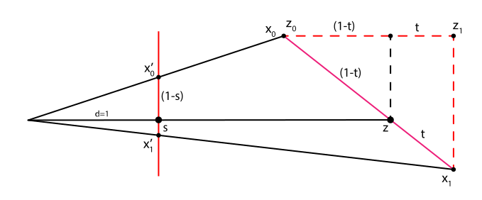
By finding the appropriate transform for said interpolation and fully simplifying it, we discover that the inverse of depth interpolates linearly in screen space. Knowing how to correctly interpolate $z$ allows us to solve for interpolated vertex attributes because the interpolation factor $t = (z - z_0) / (z_1 - z_0)$ is shared by any attribute $a$ being interpolated: $t = (a - a_0) / (a_1 - a_0)$. By equating the two, you can derive $a$. Some rearranging ahead, turns out vertex attributes divided by the associated vertex's depth interpolate linearly in screen space as $a/z = (1-t)a_0/z_0 + ta_1/z_1$, recovering the final value comes down to multiplying by the interpolated $z$. As texture coordinates are vertex attributes, we have our means for interpolating texture coordinates to pixel centers.

So, what now? Do you just point sample the texture with the correctly interpolated texture coordinates? Hahah, no. That's your one-way ticket to Aliasville. To understand why not, consider your screen. A two-dimensional grid of square pixels (assume they're square for simplicity). Each pixel has a non-zero square area. Each, thus, must faithfully represent the area of a triangle projected to it. The projected triangle area may be covered by thousands of texels all competing for the attention of the poor single pixel, depending on the geometric relationship (distance, orientation) between the image plane and the plane containing the triangle. Huge area far away or tilted in view space projects to a tiny area. In other words, the partial derivatives of the texture coordinates wrt screen coordinates at the particular $(x,y)$ are huge.

Theoretically (and ideally), we can project the screen space pixel square into texture space where it morphs into a quadrilateral which covers the texels that desire to be considered. The goal is to iterate over all the texels covered by this quadrilateral (and not one more because ✨blur✨) and filter them into a single value to be used for the pixel being lit up. As you might imagine, this is computationally expensive to do at runtime. Any kind of direct convolution like this is, by definition.

In the 80s [notably Heckbert '86], a number of solutions performed the convolution offline, but with a twist. The unwieldy quadrilaterals are hard to handle mathematically, determining whether a texel is inside or out is non-trivial. Hence, Heckbert and those before him used to replace the projection with a local affine approximation, which approximates the unwieldy quadrilateral with a comparatively-tame parallelogram or an ellipse (if you modeled pixels as circles). This was still extremely expensive for realtime use, though, but it was doable. They used a weight LUT to actually figure out how each of the texels was weighted for the final filtered value to be computed. We can't afford the convolution at runtime, at all. We need to figure out a way to precompute this. At texture creation time, preferably.

Inventing "multum-in-parvo" maps

We can approximate a projection of the screen space pixel square (or circle) to a parallelogram (or ellipse) in texture space with a linear affine approximation, the details of which are the subject of next section. While that gives us the boundaries on the texels that require filtering, it's not particularly useful to us unless we can somehow prefilter the texture. It's not feasible to cover every possible "projected" parallelogram as you can see in the sample texture below:

Those are just a few examples and it is immediately obvious that no lookup structure can be devised here. What we could do is impose some restrictions on the filter shape, for example for it to be isotropic (same in every direction) and axis-aligned:

This kind of assumption makes creating the lookup structure a lot simpler, but it will not handle anisotropy well as a square naively approximating the parallelogram-shaped filter is going to capture texels outside of the filter shape, introducing overblurring in that direction. But if you think about it, we're not limited to picking just a single square. We can approximate a parallelogram-shaped filter by doing multiple square ones placed along the line of anisotropy (the "major axis" of the parallelogram):

To facilitate this isotropic prefilter structure, known as a mipmap, we create a hierarchy of textures where each level is quarter (or half if you're looking at dimensions individually) the resolution of the previous level and the data stored in it are the filtered values of all the $2 \times 2$ blocks of the previous level. This goes all the way to a level which is effectively a $1\times 1$ texture representing the filtered value of a $\textsf{w} \times \textsf{h}$ block of the texture. Since it's square and axis-aligned, you only need the center position (basically, the texture coordinates) and a single value to access the correct levels, the width of a square of texels we're filtering.

Reducing by $4$ on each level means it reduces by $2$ in each dimension. Given a width $w_f$ of square texels we're filtering (determined in the next section), we can take the $\log_2$ of $w_f$ to get a zero-based "index" into the levels. In quotes because it can have fractional parts, for example $\log(17) = 4.087$ meaning that we have to perform two bilinear samples on levels $4$ and $5$ and then use the fractional part $0.087$ to get the final filtered value, process called trilinear filtering. Final example, say $w_f$ turns out to be $2$, it means we want to access filtered $2 \times 2$ blocks. $\log_2(2)$ is $1$, meaning we want the first level where each texel represents filtered $2\times 2$ blocks of texels of the source texture (zeroth is the source texture) and so on. As we seldom want the actual blocks that were prefiltered and closer to those in-between, we perform bilinear filtering on the $4$ nearest texels each representing a filtered block of the source texture (size of block depends on level computed).

Rounding up texels

So how do circles and ellipses work, again?

We've all dealt with circles at some point in our life, which are just a rotationally invariant kind of ellipse. The simplest formulation is usually $x^2 + y^2 = r^2$ which is trivial to understand. If you divide by $r^2$, you arrive at $(x/r)^2 + (y/r)^2 = 1$. You can see how the $r$ and $1$ on the right side constrict $x$ and $y$ isotropically from going beyond it. If you replace $r$ with $a$ and $b$, you can control the horizontal and vertical extent, effectively creating an ellipse centered on $(0,0)$ whose axes are aligned with the axes of the coordinate system:

This form is a bit bare-bones, but it gets the point across. The full, implicit equation for an arbitrary ellipse is:

$d$ and $e$ terms make the ellipse "leave" the origin and we're not particularly interested in them, so we drop them:

It can be converted into matrix form if you transform it a bit:

We have now shown that the following holds:

This is neat because we can apply transformations to our implicit ellipse parametrization as if it were any other primitive. However, there is a twist, we apply the inverse of whatever transform we have in mind. Intuition for this can be found in the way you translate something like a line to the right by actually moving the entire thing left on the $x$ term. Recall that $x$ and $y$ effectively go from $-\infty$ to $\infty$ and there's no transforming them. If we want to apply the transform $\mathbf{M}$ to facilitate $\mathbf{p'} = \mathbf{p}\mathbf{M}$, we plug in the inverse into a hypothetical ellipse $\mathbf{p'}\mathbf{Q'}\mathbf{p'}^\mathsf{T} = f'$ to yield:

We then have the transformed coefficient matrix specified as $\mathbf{Q} = \mathbf{M^{-1}} \mathbf{Q'} \mathbf{M^{-1}}^\mathsf{T}$. Also note that $f = f'$. Surely now you can see that one can start with a circle coefficient matrix (the identity matrix) and transform it into any ellipse. Further still, we can take a more generic, parametric formulation of the circle such as $\mathbf{p} = (\cos t, \sin t)$ and transform it arbitrarily then use $\mathbf{p}\mathbf{p}^{\textsf{T}} = \cos^2 t + \sin^2 t = 1$ to recover $\mathbf{Q}$ and $f$ of the implicit formulation.

Okay, now what?

What we're most interested in, though, is recovering the major and minor axis of the ellipse once we transform the parametric unit circle (representing our pixel) to the implicit ellipse using the finite difference relation clueing us in as to how texture space's $(u,v)$ changes locally with respect to screen space's $(x,y)$, our peasant-constructed Jacobian computed from $2\times 2$ blocks of pixels via finite differencing.

First things first, from the parametric unit circle to the implicit target ellipse. As mentioned, we have the Jacobian peasantly computed, so it comes down to merely transforming the points with it and recovering $\mathbf{Q}$ to get our $a, b, c, f$ coefficients:

$f$ is in plain sight, it's just the denominator. The rest of them are a matrix multiply away, just map them to the $\mathbf{Q}$ entries:

While we now have our circle "projected" to an ellipse in texture space, we need to find its major and minor axis that we'll be using for filtering (specifically, farthest points along those axes). The minor will be used to select the LOD of the mipmap and the major is our line of anisotropy we'll be sampling along at the LOD selected by the minor axis. Think back to our parametric circle prior to transform, it's a locus of points, yes? As we applied our linear transformation to it, the Jacobian, it elongated into an ellipse. There are four points on that ellipse which remained on the same two lines from the origin under the transform we performed, as if they were scaled by some value along a normalized direction which could replace the transform in that case. Yep, it's our major and minor direction "end points". This is a trivial (albeit tedious) eigenvalue and eigenvector determination problem.

Any ellipse centered around the origin can be viewed as the result of non-uniformly scaling and rotating a circle, meaning we can equate our Jacobian transform with the following:

The scaling is orthogonal while the rotation is orthonormal. As you know, the latter means rows are both mutually orthogonal and of unit length which makes its inverse equal to its transpose. Given that we define the transformed $\mathbf{Q}$ here as $\mathbf{M^{-1}}\mathbf{I}\mathbf{M^{-1}}^\mathsf{T}$, we have:

Any well-behaved $n\times n$ matrix $\mathbf{A}$ encoding a linear transform will have $n$ eigenvalues and we should be able to find $n$ linearly independent eigenvectors. If you were to place all the eigenvectors as rows of a square matrix $\mathbf{E}$ and multiplied it with the associated matrix $\mathbf{A}$ the result would be a matrix where all the rows were multiplied with respective eigenvalues $\lambda_i$... As if you had built a diagonal square matrix containing eigenvalues $\mathbf{D}$ and multiplied it with $\mathbf{E}$ yielding $\mathbf{EA} = \mathbf{DE} \iff \mathbf{EAE^{-1}} = \mathbf{D}$. Going the "other way", we have $\mathbf{E^{-1}DE} = \mathbf{A}$. This leaves us with the following equivalence:

Hence, $\mathbf{R} = \mathbf{E}$ and $\mathbf{S} = \mathbf{D}^{-1/2}$. Computing the eigenvalues for a generic $\mathbf{Q}$ amounts to:

It seems the square root and the $a \pm c$ terms will be following us around, so we might as well give them names. In the interest of keeping the result succinct, we can introduce the following substitutions $q = a + c, p = a - c, t = \sqrt{ p^2 + b^2}$. With $\mathbf{D}$, we easily resolve $\mathbf S$:

Going forward, remember that direction is our main concern, and as it aliases $\mathbf{R}$, we want them to be unit length and mutually orthogonal (a higher requirement than linear independence). Again, direction remains pristine. Thus, all shared magnitude-varying scalar factors will be dropped unceremoniously.

This nets us a pair of eigenvectors for each eigenvalue (remember the $\pm$):

Our goal is to normalize these vectors before moving forward, so let's do the first one of the first pair first... See what shakes out:

Similarly, you will find that $n_{\lambda_1,2} = \sqrt{2t}\sqrt{ t + p }$. Further, $n_{\lambda_2,i} = n_{\lambda_1,i}$ as the squaring action terminates the $\pm$ associated with $t$. But the biggest realization here is that $b$ doesn't contribute as a free term meaning that it has no bearing on the direction. We're then free to reuse the two distinct length calculations and recombine them into a single vector. Then, we can express the other vector as an implicit 90° rotation (as you know, swap the coordinates of the first one, negate one of them). This simplification will cost us some implicit sign information, but we can recover that from the sign of $b$. We have:

As we isolated a scalar factor from all of them, we can drop it because it doesn't vary the direction:

In this state, it becomes clear that the normalization factor of both is equivalent and it's $\sqrt{2t}$ which we will just prepend below. We set the two vectors as rows of $\mathbf{R}$ as it's equal to $\mathbf{E}$. Then we multiply it with $\mathbf{S}$. The rows of the resulting matrix represent the final directions for the major and minor axis.

Therefore, our final expression for $\mathbf{M}$ is:

From this we can calculate the farthest points of the ellipse along the normalized major and minor axis directions by factoring in $f$, to finalizing our boundary computation (if you can't figure out how $f$ works here, you're reading this article prematurely):

These points can be interpreted as the transformed $\mathbf{dX}$ and $\mathbf{dY}$ vectors, hence the name. Doesn't really matter what you name them, though. Whichever of the two is longer can be thought of as defining the line of anisotropy. The shorter one, its length is more important. Specifically, you need to double it to get the width of the square filter we'll be using, the $\log_2$ of which nets us the mipmap level selection value. From there, $n$ trilinearly filtered samples are taken along the line of anisotropy (defined by the other vector) and filtered into a single value. $n$ is conservative, it is dynamically determined by the ratio of the anisotropy with a maximum defined by the user (and hardware). It tries to do it with least samples, unless the count of "least samples" is greater than the maximum anisotropy set by the user / programmer. At which point, it is clamped. The spacing of the samples is determined by the hardware, how much the axis-aligned squares end up overlapping affects weighing.

And in case you were wondering, yup, this is pretty much how Direct3D, OpenGL and Vulkan perform LOD and Line Of Anisotropy determination per specification. To properly get a feel for ellipses, I suggest you use these equations we derived on a graphing tool which are usually available online, my favorite is Desmos.

GPUs have come a long way since their introduction as "3D" graphics accelerators via highly-specialized and largely fixed-function hardware. These days, they're far more general and infinitely more programmable which makes them applicable to a wide array of computing problems. Hardware companies are especially keen on this emerging market and are consciously trying to distance themselves from the term Graphics Processing Unit in favor of Compute Accelerator. The jaded among you might attribute this to a marketing ploy, but there is actual merit it. While GPUs still have some fixed function hardware within their dedicated engine for graphics acceleration, they're largely generalized and massively-parallel compute powerhouses. In fact, the majority of the conventional graphics pipeline is implemented on the back of thousands of compute cores. We're almost 15 years away from the last time we spoke of discrete vertex and pixel pipelines.

Graphics APIs and the underlying "pipeline" have, unfortunately, failed to keep in lockstep with the evolution of GPUs, mostly out of comfortable complacency because the classic IMR graphics pipeline is, more or less, a success story which delivers great performance for everything but the most demanding of applications. To push boundaries beyond what's comfortable, Independent Hardware Vendors, Independent Software Vendors and platform holders have come together to enable next-generation graphics APIs such as Direct3D 12 and Vulkan in the mid 2010s. Even with all these advances, a big part of pushing more detail on screen remained in limbo, restructuring the geometry processing pipeline. For the past few years, this has been the hot topic among realtime computer graphics researchers.

The fruits of said labor have been available for two years at least, but adoption in the mainstream will be a tenuous one. This is especially true of personal computers where graphics hardware prices have been skyrocketing due to Nvidia's de facto monopoly. Today, I am going to give you a tour of what you can expect on the PC and, of course, Xbox Series X which will come with full support out of the (x)box. The same is true of PlayStation 5, which should help early adoption because AAA developers use consoles as a baseline and PCs as port targets.

Why change?

The coarse diagram found below this paragraph should be old hat to you by now. It is a high level overview of a basic IMR architecture with one of its crown jewels, the ubiquitous vertex shader. For simplicity, it's missing tessellation and geometry shading stages. We'll get to the former in due time while the latter should be bleached out of your mind.

A vertex shader, at its core, is nothing more than a wrapped compute kernel with special semantics and output requirements, executing on many cores. What predicates thread dispatch and data shoveling is, in D3D parlance, the input assembler stage.

Hardware companies have their own designations for the piece of fixed-function hardware associated with this stage, we will adopt Nvidia's terminology for the duration of this article. On Nvidia Pascal GPUs and below (Maxwell, Kepler, Fermi...) it is known as the Primitive Distributor which is a fairly apt name given that it takes the inherently serial index buffer and determines the best way to cut up (distribute) the supplied vertex buffer into batches which maximize utilization and on-die memory sharing once thread dispatch begins.

Once vertex processing ("shading") is finished, the next piece of fixed-function hardware hit before the rasterizer is the viewport clipping (and culling) stage. It takes the processed vertices and, as the name implies, performs fast clipping and culling operations against the configured viewport. While it is very good at what it does, it is preferable to perform culling before processing vertices. Like with the primitive distributor, fixed-function hardware needs to step down a bit in the interest of flexibility.

How the Primitive Distributor hurts you

First thing I need to impress upon you is that index buffers exist to avoid vertex duplication by generating index duplication. Depending on representation, indices can be as wide as \(32\) bits. Therefore, this is extremely wasteful during processing. To illustrate what the primitive distributor does, let index buffer \(\mathbf{IB}\) for primitive_topology::triangle_list contain the sequence of indices [7123, 7124, 7125, 7123, 7124, 7126, ...]. From here, we need to isolate the unique vertices referenced into a batch \(\mathbf{B_v}\) as [7123, 7124, 7125, 7126, ...], bear in mind we use the original indices to refer to the vertices for readability. Original because for every such vertex batch, a special primitive indexing batch is generated relative to it, allowing indices to be represented with significantly fewer bits (such as $8$ bits), \(\mathbf{B_i}\) as \([0, 1, 2, 0, 1, 3 \space ...]\).

Given that thread dispatch granularity on Nvidia GPUs is 32 threads (the size of a warp), to maximize utilization and performance, the primitive distributor will try to fill up as many 32-wide vertex and primitive batches as possible. While this gives you a clue on why processing tiny vertex buffers is quite expensive on a large scale, the real performance culprit is the fact that said index deduplication is performed every frame, dozens and even hundreds of times a second. That's bad, especially in the case of static geometry.

What are we to do?

Further embrace the compute accelerator nature of modern GPUs. Modify the hardware in such a way that it doesn't hinge on the Primitive Distributor and the misplaced viewport clipping/culing stage. The classic graphics pipeline can be implemented in terms of the more flexible system which doesn't have a set number of stages and it can be done by the runtime and the driver for backwards compatibility for the many people who can't beat the fixed function hardware on their own.

Don't do unnecessary work. Primitive Distributor's work can be largely kicked off to a build/bake step in the engine. Fundamentally, the Primitive Distributor will break up a mesh every time into a bunch of meshlets which are going to run in waves. The Primitive Distributor is also not magic, if your topology is trash, performance will suffer. Once it's relegated to a bake step, a lot more time can be spent on optimizing the meshlets for online processing, shortening the path to the rasterizer at runtime.

Arbitrary geometry representations follow naturally as you no longer have a requirement of providing conventional vertex and index buffers, allowing for novel and compact representations.

Amplification & meshlet shaders

As discussed in the last section, threads are dispatched on a hardware-specific granularity within which it is possible to share data and perform otherwise unavailable performance-enhancing operations known as wave intrinsics. Thus it's necessary to optimally break up a mesh into cache-friendly meshlets at bake time (as opposed to runtime). Furthermore, issuing thread groups sequentially, once per-vertex followed by an optional per-primitive stage is not very flexible. It is preferable to intermittently operate on both per-primitive and per-vertex data within each thread of execution in order to maximize opportunities to avoid work. As the old addage goes, the most performant operation will always be a NOP.

(De)amplified meshlet killed the vertex star

One thing that made vertex shaders such a success story was the tremendously simple programming model. Vertex comes in, processed vertex comes out. Geometry shaders are similarly simple as they perform work on a per-primitive basis. While they were a good-ish idea on paper, executing threads on a per-primitive basis and doing so after the fact is a somewhat limiting factor... Doubly so because anything a geometry shader can do, a compute shader can do better. Thus, it made sense to offer an alternative to vertex and geometry shader combos in the form of the novel mesh(let) shader. To account for tessellation, culling and instancing concerns, an aptly-named amplification shader precedes the meshlet shader which potentially amplifies or "dampens" input geometry while allowing early removal of offscreen surfaces before any expensive per-primitive and per-vertex processing takes place. In Nvidia parlance, it is also known as the task shader.

Put simply, the amplification shader determines just how many mesh(let) shaders will have to be executed. Remember how I told you that most of the graphics pipeline is basically a bunch of wrapped compute shaders with intermittent fixed-function stages? You can see it here clearly as now you have access to shared memory which means the usual thread-addressing IDs are fed into the shader (in HLSL, these would be sysvals such as SV_GroupThreadID and SV_GroupID). As the meshlet shader needs to produce some useful output, you have to write to two arrays, one for per-vertex data and the other for per-primitive data. There is flexibility in how much data you write but upper bounds must be specified ahead of time.

Just like D3D12 offered the developer more control over the GPU by having the runtime and driver step aside for you to make your own trade-offs, tessellation in the conventional sense is gone in this new model. This is good because the fixed-function tessellator has a predefined and immutable pattern used to generate more detail based on the hull shader's constrained output. Nowadays, for better or worse, both the inputs and outputs for tessellation are user-defined.

At this point, I am hoping it is becoming clear to you that this added flexibility may very well mean a performance catastrophe if you don't know what you're doing. Beating old fixed-function hardware is only possible if you know what you want and are willing to go above and beyond when it comes to availing yourself of the new programming model, especially taking advantage of the ability to perform culling ahead of time. If else, don't use this. If you are thinking of redoing the classic geometry pipeline in terms of amplification and meshlet shaders, you're missing the point.

The nitty-gritty details

Amplification and meshlet shaders are easier to define in terms of their limits than their possibilities. It should be very clear to you by now that there is no catch-all code snippet I can give you to put into your application. With that caveat in mind, here's a simple, non-production, introductory meshlet shader in HLSL for you to get a feel for things:

// I hate CamelCasing.

struct ThreadInformation {
    uint3 ID                    : SV_DispatchThreadID;
    uint3 GroupRelativeID       : SV_GroupThreadID;
    uint3 GroupID               : SV_GroupID;
    uint LinearGroupID          : SV_GroupIndex;
};

[numthreads(64, 1, 1)] [outputtopology("triangle")]
void processMeshlet(in ThreadInformation threadInformation, out vertices Vertex outputVertices[64], out indices uint3 outputIndices[126]) {

    // Structured buffer, probably
    Meshlet meshlet = meshlets[threadInformation.belongingGroupID.x];
    SetMeshOutputCounts(meshlet.vertexCount, meshlet.primitiveCount);
    uint linearGroupRelativeID = threadInformation.LinearGroupID;

    // Per-vertex processing
    if(linearGroupRelativeID < meshlet.vertexCount) {

        // Get the associated vertex index and read from yet another structured buffer
        Vertex vertex = vertices[meshlet.vertexOffset + linearGroupThreadID]; 

        // ... Do your vertex processing.

    }

    // Per-primitive processing
    if(linearGroupRelativeID < meshlet.primitiveCount) {
        // Similarly, process and assemble primitives, store result into outputIndices.
    }

}

You will need to upgrade your compiler to get this to work, FXC has now been surpassed by DXC. While HLSL is still a soaring dumpster fire, it's actionable. Can't hold a candle to the C++14-based Metal Shading Language, though. However, with the advent of SPIR-V and going from DXBC to DXIL (thanks, Clang), you can produce your own shading language that does exactly what you want it to. Note that using FXC generated DXBC will incur load-time conversions to DXIL behind the scenes.

How do amplification and meshlet shaders "talk"?

In in DX12 Ultimate / HLSL parlance, we have payloads which are at most 16 KiB worth of data per triggering meshlet shader and is used instead of explicit structured buffers in the example above. Instead, those are moved to the amplification shader where input decoding of your custom geometry format is performed followed by culling computations of arbitrary complexity, tradeoffs are yours to make. A skeleton looks like this:

struct Payload {
    // User-defined and arbitrary, sky is the limit (16 KiB)
};

[numthreads(64, 1, 1)]
void prepareMeshletDispatch(ThreadInformation threadInformation) {

    Payload meshletPayload;

    //  Decode your geometry format, cull, prepare tessellation and instancing. 

    // Then dispatch a fresh meshlet for processing:
    DispatchMesh(numberOfThreadGroupsToDispatch, 1, 1, meshletPayload);

}

[numthreads(64, 1, 1)] [outputtopology("triangle")]
void processMeshlet(in ThreadInformation threadInformation, in payload Payload meshletPayload, 
                    out vertices Vertex outputVertices[64], out indices uint3 outputIndices[126]) {

    // Use whatever your payload is to generate work for the rasterizer

}

Again, how you write these two will highly depend on what kind of application you have. Careful thought and testing will be required to determine whether you benefit from this new approach at all. Don't pull a Deus Ex: Mankind Divided where the D3D12 implementation actually had worse performance than the D3D11 one.

How do I access this from the API?

Once this hits the API, a new method on the graphics command list interface will be available:

void ID3D12GraphicsCommandList6::DispatchMesh(UINT ThreadGroupCountX, UINT ThreadGroupCountY, UINT ThreadGroupCountZ);

Similarly, indirect meshlet dispatching will be supported via the upcoming D3D12_INDIRECT_ARGUMENT _TYPE_DISPATCH_MESH enumeration and D3D12_DISPATCH _MESH_ARGUMENTS structured member. As you can see, the majority of the big brain time will be sequestered inside of your geometry encoding scheme, meshlet preparation and the amplification and meshlet shaders.

out primitives PerPrimitiveData outputPrimitives[PRIMITIVE_COUNT_MAX]

Multum In Parvo

My preferred way of thinking about clipmaps is in line with Tanner et al. A clipmap is, for all intents and purposes, a virtual mipmap. Therefore, we shall first refresh ourselves on the merits of mipmaps and smoothly transition from there.

As you probably know, textures slapped across geometry come in a variety of sizes. Even the practical upper limit for non-virtual, fully resident textures is a staggering 16384x16384. These objects often end up projected to a very small area on the screen, invariably leading to aliasing as there may be thousands of texels competing for a single screen pixel. One could, ludicrously, filter this at runtime every single time... Or realize all of this can be precomputed at texture creation. Enter the mipmap.

A mipmap ("Multum In Parvo" means "much in little space") is a hierarchical structure representing a source texture (conventionally and historically, a "bitmap"). Each level is half the resolution of its predecessor, all the way down to 1x1. Any filter can be used to perform the downsampling, even a 2x2 box filter. A precomputed solution to avoiding aliasing. Mipmaps also have secondary interpretations which are equally valid. One is that they inherently serve as a texture level-of-detail solution which alleviates bandwidth issues by only accessing the optimal resolution of the texture wrt what can be seen given the camera distance to the surface.

This immediately leads us to the motivation behind clipmaps. Consider the opposite scenario. When the source texture is massive (eg. 65536x65536) and covers a large element in the game world which seldom (if ever) fits inside the view frustum (think terrain, planets, world-spanning acceleration structures), only aperture-sized parts of a mipmap are actually utilized and the available memory should be focused on those rather than being wasted on stuff that's offscreen at the moment. Thus, if one dynamically "clips" off the unneeded sections of the mipmap, you essentially convert an inherently static mipmap pyramid into a dynamic clip stack with a residual, potentially static mipmap pyramid stump, collectively known as a clipmap.

Each level of the clip stack has exactly the same amount of texels which means, when centered against the corresponding mip level of a mipmap, the extent will increase as you go towards the bottom. Once the extent becomes 1:1, it collapses back into a residual mipmap pyramid which is small enough to be constantly in memory. This is conventionally expressed as two separate resources in software, clip stack is represented as a texture array which is updated high-to-low from the CPU (streaming) while the residual mipmap pyramid is a potentially static, regular mipmapped resource.

As mentioned, given the top (level 0) of the clip stack has the same amount of texels as the bottom, it covers the smallest area of the source texture. This is intentional because even with oblique viewing angles, the perspective transform squashes and minimizes stuff in the distance, large areas in world space project to very small areas in screen space (mipmap's specialty). The classic mip level selection would actually try to sample individual clip levels out of bounds. Thus, we require an additional mechanism to account for selecting a proper clipmap level for the logical texture address.

How does it work?

Naturally, the first thing that comes to mind is the clipmap update/streaming method. Every time you move, you offset everything to the side and all of it seemingly needs to be overwritten. However, consider moving just a little bit in any direction. Due to the coherency of the data in the mipmap, you only need to replace the parts of levels of the clipmap that are now outside of view. By moving the origin of the clipmap to the center and engaging the address_mode::wrap, you can actually load what's supposed to be on the right on the left side. The same works vertically. And is separable. This addressing is called toroidal in academic circles and is showcased below.

Selecting the correct clip stack level

With all of this in mind, we define $l^s(d)$ as $\log_2(ksd)$ and look for $k$ which satisfies our requirements such as $l^4(0.125) = 1$:

This finalizes our minimum clip stack level selection function as:

You compute both the vertical and horizontal level and choose the "worse" one. In case you haven't been paying attention, that's the larger one with less detail and higher extent. And in the end, you also compute the regular mipmap level selection and compare it against the clip stack level selection. Picking the "worse" one ensures there is neither aliasing nor out of bounds accesses. The attentive among you may notice that $l^s(d)$ dips below $0$ for some values. But then again, you also noticed that once we necessarily $\max$ it against the mipmap level selection function, the issue is eliminated.

Transforming coordinates for final clip stack sampling

A recap of recent history

In the early 2000s, central processors were still single-threaded and GPUs were considerably less programmable than they are today. The solution was introduced in the form of special hardware functionality to tackle occlusion culling on the GPU called "hardware occlusion queries". However, they require a ridiculously slow, error-prone, constant ping-pong match between the CPU and the GPU which considerably reduces the possible performance gain margins. The CPU has to configure the GPU for occlusion queries, submit the query data (render coarse geometry) and read back the results in order to update its indirection-heavy hierarchical structures dedicated to accelerating visibility determination and avoiding false negatives. And only then is it finally able to submit all the visible instances for rendering using the immediate mode APIs of the time (Direct3D 9.x / OpenGL 1.x+). The most successful approach of this generation of occlusion culling technology was called coherent hierarchical occlusion culling (commonly abbreviated as CHC++).

Coherent hierarchical occlusion culling in action

Sliding into the 2010s, more and more users had already acquired multithreaded microprocessors which boasted vectorization extensions as well. Tired of the cache-incoherent nature of hierarchical occlusion culling, hard-to-manage false negatives and overall latency of communicating back and forth with the GPU before even beginning to construct a frame, we turned to more CPU-centric, data-oriented methods for occlusion culling. Especially as it was already becoming more and more economical to just brute force "general" culling just by doing view frustum culling against large blocks directly on the CPUs and still run circles around methods like octree-based culling. The solution was a bit out there, we're essentially talking about software occlusion queries. They involved running a small rasterizer on the CPUs which generated a low resolution depth buffer which would then be used solely with bounding geometry to estimate occlusion by large, predefined static occluders. First commercially successful game (I am aware of) that opted for this method was DICE's Battlefield 3 running on the Frostbite engine. I have no doubt that this was directly motivated by the considerable number of Cell SPEs alongside the PPU on the Playstation 3.

Software-rasterized low resolution depth of large, static occluders for occlusion testing.

With the arrival of true indirect dispatch allowing the GPU to compute the drawing set on its own without CPU intervention, a shift back towards hardware-accelerated occlusion culling was made. This was further bolstered by advances in temporal reprojection approaches, leading to methods where the occlusion culled set was determined using a downsampled, hierarchical depth buffer from previous frames during the advent of "next-gen" graphics APIs around 2014 and 2015.

Around that time, I had a strong itch regarding whether or not I could mix early-z testing and conservative rasterization to utilize fast hardware paths of modern GPUs to do my occlusion culling for free because there are penalties to the hierarchical approach which I deemed undesirable. Unfortunately, conservative rasterization tier support on modern GPUs was and is so bad that even Maxwell 2.0 GPUs like the GTX 980 support only tier 1 which is inadequate for the task at hand. On the other hand, my hunch about early-z subversion was right on the money. And fortunately for me, I wasn't the only one to consider it which is always helpful to avoid a considerable amount of head-scratching and writing suboptimal implementations.

Are you still there?

// Optimized for readability
#define THREAD_GROUP_DIMENSION 8

// Organize your data as you like.

struct thread_execution_information {
    uint3 thread_id : SV_DispatchThreadID;
    uint3 thread_group_id : SV_GroupThreadID;
    uint3 group_id : SV_GroupID;
    uint group_index : SV_GroupIndex;
};

[numthreads(THREAD_GROUP_DIMENSION, THREAD_GROUP_DIMENSION, 1)]
void main(thread_execution_information executing_thread_information) {

    float2 const center_offset = float2(0.5f, 0.5f);
    float2 const thread_fid = float2(executing_thread_information.thread_id.xy);
    float2 const downsampled_buffer_dimensions = 0.25f * depth_buffer_dimensions;

    // This will move us to the center of each 4x4 block within the full resolution buffer.
    float2 const downsampled_center = (thread_fid + center_offset) / downsampled_buffer_dimensions;
    if(downsampled_center.x >= 1.0f || downsampled_center.y >= 1.0f) return; // Out of bounds

    // Full resolution buffer texel size, so we can get to the centers of the surrounding
    // 2x2 blocks on which we will apply D3D12_FILTER_MAXIMUM_MIN_MAG_POINT_MIP_LINEAR,
    // to ensure there are no zero weights which would discard them from the max comparison.
    float2 const full_resolution_texel_size = 1.0f / depth_buffer_dimensions; 
    
    float block_maximums[4];
    float2 block_center_offsets[4] = { 
        float2(-1.0f, -1.0f), float2( 1.0f, -1.0f), 
        float2( 1.0f,  1.0f), float2(-1.0f,  1.0f) 
    };

    [unroll]
    for(int i = 0; i < 4; ++i) {
        float2 const center = downsampled_center + full_resolution_texel_size * block_center_offsets[i];
        block_maximums[i] = depth_buffer.SampleLevel(depth_max_sampler, center, 0).r;
    }

    // Final manual maximum determination performed, ready for reprojection.
    float downsampled_depth = max(max(max(block_maximums[0], block_maximums[1]), block_maximums[2]), block_maximums[3]);

    // ...

    // We're in texture space right now. In Direct3D, the origin is the top-left corner.
    // In order to use the inverse projection transform, we need to go back to normalized device coordinates.
    // Depth is in the 0 to 1 range, Y axis is flipped and XY go from [-1, 1].

    float2 xy_ndc = downsampled_center * float2(2.0f, -2.0f) - 1.0f;
    float4 position_ws = mul(previous_inverted_projection_view_transform, float4(xy_ndc, downsampled_depth, 1.0f));
    position_ws /= position_ws.w; // Complete the non-linear part of the transform.

    // Using the new world position and the current projection-view transfrom, we compute 
    // the new placement position in texture space to put the reprojected depth in.
    
    // First to NDC:
    float4 reprojected_position = mul(current_projection_view_transform, position_ws);
    reprojected_position /= reprojected_position.w;
    float depth = reprojected_position.w < 0.0f ? downsampled_depth : reprojected_position.z;

    // Then to texture space:
    reprojected_position.xy *= float2(0.5f, -0.5f); 
    reprojected_position.xy += 0.5f;

    // The downsampled depth buffer has all its values initialized to 0 by default, which precludes the possibility
    // of utilizing InterlockedMin, requiring us to do some inversion gymnastics here for this to work.

    uint intermediate_depth = asuint(1.0f - saturate(depth));

    // Safest thing is to overwrite the possible hole immediately, minimizing the error (but this is a coarse approximation)
    InterlockedMax(downsampled_depth_buffer[executing_thread_information.thread_id.xy], intermediate_depth);

    // Finally store in reprojected position as well.
    int2 reprojected_position_ps = int2(saturate(reprojected_position.xy) * downsampled_buffer_dimensions);
    InterlockedMax(downsampled_depth_buffer[reprojected_position_ps], intermediate_depth);


}

RWStructuredBuffer<uint> visibility_buffer : register(u0);

[earlydepthstencil]
void main(uint instance_id : SV_InstanceID) {
    visibility_buffer[instance_id] = 1; // Free lunch.
}

Approaching the problem...

Shuffle it around a bit, into a form where we'll be able to scam the integral into doing what we want. Just to emphasize for those who get bamboozled by the following sausage is that it is just $E_{\mathbf{multi}}(\omega) = 1 - E_{\mathbf{first}}(\omega)$ laid bare:

We need to fit a function $\rho$ which will resolve the left side to what we see on the right side, as such, it can be expressed as a product of a currently unknown number $N$ of factors, each potentially a function of $\omega$ and $\omega_i$:

It is not hard to guess what our first factor will be, pretty much the right side which will allow us to focus on forcing the integral to dissolve:

To get a grasp of what's going on, we're going to change our variables to deal with the unit hemisphere in a way which is directly computable. Furthermore, we also dole out the normalization factors necessary after we process the outer integral:

Now, you might be tempted to guess the remainder of the product defining $\rho$ right away, to be something along the lines of:

Cheeky, but no. You may be scratching your head as to why. You've just added a portion of the parametrization of the integral into the denominator of our multi-scattering function and its respective normalization. Change the variables from $d\theta_i$ to $du_i$ where $u_i(\theta_i) = \cos\theta_i$ and watch the house of cards crumble. Awkwardly floating sine alongside now irrelevant normalization factors. How about something like this instead:

This was something I could precompute and put in the denominator as a normalization factor alongside $2\pi$, in my initial approach. While my intention was not to give any particular semantics to this particular integral, it looked like a weighted average of the albedo where the weights were a function of the cosine of the angle (essentially direction where light is shot out)... It's just missing the weight scaling factor:

And we can pretend the $2$ out of our normalization is the weight scaling factor, just call it $\bar{E}$:

What of the Fresnel factor in this approximate multiscattering framework?

Putting it all together

With all of this in mind, we can now augment any microfacet BSDF with an energy compensation term which is essentially approximating multiple scattering:

In the next article, we'll be covering how the integrals are precomputed and/or fitted into the budget of a realtime application (pun intended), especially incorporating Fresnel into the mix in a way where the look-up tables won't be "unnecessarily multidimensional" and prohibitively expensive. As it stands now, it's non-trivial to compute, to say the least. To give you a taste of what we'll be doing, here's the albedo function of the single-scattering microfacet BSDF (with $F=1$) encoded as a two dimensional image (horizontally a function of angle, vertically a function of roughness):

$E_{\mathbf{first}}(\omega)$ precomputed into a 2D texture. You could even get away with a LUT as small as 16x16 given how smooth it is.

We'll have to roll up our sleeves to get Fresnel into the equation (pun intended) in a way that isn't at odds with practicality that a realtime system needs. Once we finalize that, we will jump into the work of Turquin who had a pretty interesting hot take on an approach of this flavor (of which Sony's Imageworks people are also proponents of)... He, interestingly, opted in to variably scale the single-scattering BSDF instead of manually developing a secondary term like we just did. And if you'd like to see a "before/after" image, I've got you covered:

The difference is rather striking at high roughness!

The furnace differential at high roughness is the best argument for approximating multiscattering.

With the ever-increasing pixel density of modern displays and the less than satisfying didactic coverage of vector graphics, there's been growing interest among my colleagues regarding my hardware-accelerated implementation. In this article, I will attempt to quickly outline a simplified, scanline-based approach I implemented for use with my custom GUI framework and, by extension, Police Line. Modest knowledge of Bezier curves is a prerequisite for the reader, some of which can be acquired in a previous article.

Commercial and academic state of the art

Whenever I mention I wrote a custom, online vector graphics rasterizer, most guess it is based on ideas developed by Loop and Blinn in 2005 or Kerr in 2009. Alas, both approaches require runtime CPU-based precomputation which easily becomes the bottleneck when processing complex vector graphics.

The former triangulates the path vertices on the CPU to generate geometry that represents the filled interior while parametrically solving the partially covered boundary in what is effectively texture space on the GPU. The latter, used in Direct3D 11-based Direct2D, is not entirely dissimilar as it revolves around converging to the path interior through trapezoid tessellation, a costly step performed, once again, on the CPU. Which is to say, both guesses are wrong.

While there have been developments as late as 2019 which propose generalizing 2D patch primitives suitable for GPU processing, they still require a hefty precomputation of whichever paths one desires to rasterize. Managing that doesn't seem particularly enticing given that the resulting speed-up is not necessarily stellar compared to my preferred approach, parallelizing the conventional scanline method. I reckon the most recent paper on the parallelized scanline rasterizers was written by Li et al. in 2016.

The paper, while interesting, has issues. It somewhat tends to hand-wave away important details, implies more complicated mechanisms are at play than in actuality and the supplementary code is fairly bad, even for academics. To add insult to injury, the provided reference implementation is written against the vendor-locked CUDA which is hardly appropriate for a purported solution to a real world problem.

Vector graphics in the game industry

Current commercial landscape is also rather sad, the middleware of choice for AAA studios, Scaleform is notoriously expensive and slow with games such as the latest Spiderman burning up to 8 ms on the UI alone. Microsoft's Direct2D, as outlined by Kerr in 2009, has an expensive CPU-side geometry generation and tessellation step and, as an API, is almost universally hated. With the advent of Direct3D 12, it cannot be used without serious issues and complications that arise from the Direct3D11on12 "translation layer" as it was built on top of the traditional Direct3D 11 API. Once and if you try to combine it with DirectComposition, it pretty much implodes.

Scaleform in Borderlands

On the other end of the spectrum, offline rasterized UI graphics at multiple resolution "LoDs" seems to be the nominal approach for apps on Apple devices, but also many a game. The latter sometimes just cover the bare minimum (96 dpi) which makes returning to them later a blurry mess.

There are also alternative solutions that are neither here nor there suitable for text rendering, based on signed distance fields. To my knowledge, applying SDFs to text rendering was popularized by Valve back when they were still making games and is actively used today by at least Unreal Engine 4.

Parallelizing the scanline

In the conventional, horizontal scanline rasterization method, the idea is to sweep along the raster grid vertically, intersecting with path curves at each iteration and filling in the spans in-between according to the fill rule (even-odd or non-zero) applied to the accumulated winding number wrt any position on said span. Naturally, this requires the intersections to be ordered. For the longest time, this has been impossible to do on the GPU efficiently due to the method's sequential nature and complex, prolonged computations. It's not any one thing we devised in the meantime as much as it is the increased programmability of GPUs that made it possible. Not only are GPU programs now able to be much more expressive, they can also be far longer as instruction count limitations have virtually been removed.

Key observation one needs to make is that the spans between two sequential scanline intersections with curves belonging to the same path all have the same winding number and can be processed as a unit, ie be indirectly scheduled as a hardware-accelerated line draw. More importantly, these spans are completely determined by the two intersections on either end. Specifically, the pixels on the span boundary containing portions of said curves. We shall use OpenGL vernacular and call these boundary/edge fragments as multiple paths may go through the same pixel. It quickly becomes clear that accumulating all those fragments by intersecting all the individual curves with the pixel grid will set the foundation for our rasterization method.

As multiple curves may land onto the same pixel and generate separate boundary fragments, we will also need to merge fragments that intersect curves that belong to the same path as they need to be processed as a unit. As the paths do not necessarily cover every pixel grid line, it would be wrong to run a thread for every grid line. Our parallelization basis for this stage will thus be the individual curves of each path. This may set off a red flag for you. Rightly so, curves that are way too long will intersects thousands of grid lines. As a bake step, you can convert any long path curves to shorter curves as a function of arbitrary heuristics that are up to you and your project's needs.

At this stage, we need to perform numerical root finding to test each relevant grid line against each individual curve dispatched. Most root finding algorithms for "online usage", including the simplest bisection solver, require an interval where samples at the limits have opposing signs. To achieve this, we need to have the curve extremities parked within the axis aligned bounding box of each curve's start and end position to enumerate and process the relevant grid lines without multiple intersections. We need to guarantee convergence for the bisection solver. This means that our inner control points, the tangents, need to be within the said bounding box. In other words, making sure every grid line "within" the bounding box intersects the curve and intersects it once.

We do this by making each curve monotonic, ie only increasing or decreasing wrt either axis. Naturally, we seek the roots of the derivative of each curve to find positions where this trend is broken (ie $t$ where the derivative is $0$ wrt $x$/$y$, indicating a tipping point for the curve). For linear curves (lines), they're already monotonic and we do no work on them. Quadratic curve's derivative is linear, trivial to determine whether it intersects 0. Cubic curve's derivative is quadratic and there is the "famous" solution to find the roots (zero). We collect all these curves and test them against the relevant lines using a bisection solver, this way we can initialize the next iteration from the previous by iterating over the grid lines one-by-one. In the end, we combine the individual $t$s and sort them to get pairs of intersections whose middle will reveal the location of the newly generated boundary fragment.

After accruing the boundary fragments, we need to sort them to actually generate spans between them and separate them by scanline, to allow us to compute the winding number on each of them. We do this by performing stable sorts against the individual coordinates of the boundary fragment as well as the path ID to make sure the "painter's algorithm" is maintained. We also merge all the boundary fragments belonging to the same path ID and pixel. At this point, we can process each merged fragment on its own by running a line through the center and checking for intersections with the constituent subcurves. Depending on the direction of the curve, clockwise yields $1$, counter-clockwise yields $-1$. Once all the merged fragments have this small computation done, we can use a prefix sum (specifically, an exclusive scan) to calculate the winding numbers at each of the possible spans between them. Anywhere where the resulting prefix sum is odd or non-zero (according to whatever fill rule you choose), you render the span between the $i$th and $i+1$th fragment's location, if they're on the same scanline (non-inclusive).

Merged boundary fragments require special attention to actually get to the sample points. By extending vertical and horizontal "rays" (really line-curve tests, rays are merely descriptive) and counting crossings, we determine whether any of the MSAA sample points is covered or not (same deal, $0$ or $2n + 1$). In the end, you manually fill in MSAA coverage information and render all the boundary fragments indirectly as 1x1 lines.

Potential for precomputation and further optimization

The vertical and horizontal line-curve crossing tests for samples are separable and can be precomputed individually for all MSAA samples, stored into lookup tables. The vertical component is solely a function of the individual curve's intersection with the left edge of the boundary pixel. Horizontal is more complicated, but you can arbitrarily approximate each subcurve with lines going through the start, end and $n$ interim points. By deriving the half-plane from each such line, you can precompute and lookup the bitmask of all samples on the relevant side of the line. By repeating this for each line approximation and closing off the top and bottom, a bitwise and will give you the final bitmask. This is linearly combined with the vertical lookup and the main ray to get the final bitmask for the boundary fragment, to be used to fill out MSAA coverage when rendering the 1x1 line representing the fragment.

Fun. Got to go. Bye.

Properly configuring and handling a swap chain is crucial to ensuring a responsive and pleasant interactive application. Whether you're developing a digital content creation tool, video playback software, simulation or game which requires fluid controls, there's a lot to configure in order to ensure smooth sailing. Unfortunately, rich options and poor documentation often mix poorly and result in mediocre performance, bordering on bad. This is further exacerbated by the lack of a silver bullet configuration, as each application has its own specific needs which map it to a different location on the throughput-latency trade-off chart.

Things have changed

Exclusive fullscreen mode, in the traditional sense, is gone in Windows 10. People are still polarized on the subject, I personally find it to be a step in the right direction. Anyone who owns a multi-display setup sighed in relief when they first noticed that Alt+Tab no longer resulted in epileptic blinking due to mode switching. Who could forget the agony of having your system gamma settings messed up or games crash after switching to another application because they weren't programmed to recover from an unsolicited mode change instigated by being put in the background. A game is an application like any other and the experience should be as smooth, if not smoother.

So, why isn't everyone onboard? Everything on Windows 10 is presented to the screen solely through the compositor, a key component of the Desktop Window Manager. To ensure there is no tearing when presenting a buffer to the display, the swap happens exactly at the time of a vertical blanking of the screen (usually, every 16.67 ms). A non-negotiable* V-Sync. Unfortunately, somewhere along the way bad programmers happened and introduced a massive amount of input lag by misunderstanding how the swap chain behaved with V-Sync enabled which started a decades long prejudice against V-Sync among gamers, all thanks to a few popular, but technically inept games.

Gamers disabled it altogether and lowered settings to a point where they could consistently hit 200 frames per second. They ignored the screen tearing and the drop in rendering quality because it gave them a spring in their step in-game as all the unnecessarily computed frames were just discarded and the latest one was used, holding their newest inputs. As a developer using fullscreen exclusive mode, you didn't have to justify yourself to DWM, you would just say: "Here's the fresh buffer, read from it, I don't care if you were in the middle of another buffer." And... It's gone. Someone's bound to be upset.

The root of V-Sync prejudice

Why do some games have ridiculous input lag with V-Sync enabled, even when they complete frames in less than 16 ms? Generating a frame for any modern game running on a computer with recommended specs does not actually take less than 16.67 ms, no matter what the Steam FPS overlay tells you. The GPU time tells only a part of the story. CPUs are required to read inputs, update state and then define, encode and enqueue all the work that needs to be peformed subsequently on the GPU to get a complete frame to present to the screen. Optimally, this happens in less than 16.67 ms. So, if you were to press the move key right now in an optimal game (CPU time: 16ms, GPU time: 16ms), in the best case scenario your changes would be registered in just over 33 ms, hitting the (relative) second vertical blanking event provided that the CPU work began at exactly after the last vertical blanking event. To understand this a bit better, let's start "at the bottom" and work our way up.

With the approach outlined in the example diagram above, the CPUs are yawning while the GPU is filling Buffer 0. The solution to this is to introduce pipelining. The CPUs can begin work on a new frame immediately after a present is queued (implicitly by calling IDXGISwapChain1::Present1). This doesn't reduce latency, but it does increase throughput. Until now, we have only allowed a single present to be queued, hence why the CPUs didn't start working on the next frame immediately. This is the implicit minimum frame latency of 1. To allow for pipelining, we need to allow for at least two presents to be queued (our maximum frame latency) and match the numbers of available back buffers. Otherwise, we'd have to wait on a surface to become available. By default, which is what a lot of people use, the maximum frame latency is 3. We don't necessarily have to hit all 3 presents, these settings are there to ensure a smooth framerate at the expense of latency when hiccups happen. Hiccups are a result of deviations in CPU and GPU times combined with the shifting phase of CPU work with respect to a blanking event, incurring a miss of the next vertical blanking event as demonstrated in the image below.

While this has been neatly set up to happen right at the start for demonstration purposes, this will happen. The phase of CPU work with respect to vertical blanking events changes every frame and both CPU and GPU workloads vary from frame to frame, a third present will eventually find its way into the queue and demand its time on the screen. After that happens, it is highly unlikely a three frame latency will be undone (and even if it were, it would just happen again). Which increases your average baseline input latency to just over 50 ms. Furthermore, if a buffer is being used on screen, the GPU cannot proceed to work on it. This results in the GPU having gaps in the timeline as it delays work beyond the next blanking event, when the current front buffer's time is up. You might be thinking: "I'll just have 3 back buffers and that will fix it." That would actually only make things worse. Once the present queue is full, you will be able to encode the next frame, but once you inevitably attempt to present, you will cause a block inside of IDXGISwapChain1::Present1. It waits until the queue is reduced by one (next vertical blanking) and then inserts it at the end, returning back to user code. This vicious cycle would continue with frames constantly queueing after blocking, earning you an additional 16.67 ms latency penalty for a grand total of just over 66 ms on average.

50-60 ms is the usual input latency incurred by misunderstanding swap chains (usually leaving them on default), and that's when you're aiming at a compute budget that is less than 16 ms on both the CPU and the GPU. Games that are locked to 30 FPS (budget being 32 ms for each), you usually get more than double the latency. And this is just your baseline, self-inflicted input lag. On top of all this, there is the constant 60-80 ms latency of having the actual image transmitted and displayed on the screen. Console gamers have been living with latency reaching 200 ms for years. Most PC gamers feel comfortable with latency being around 100 ms, although they have no idea it's actually so high, they gauge it by feeling it. In the next section, we discuss how to bring baseline input latency down to 33 ms for games aiming at 60 FPS games without tearing (or 66 ms if you're going for 30 FPS, nobody's judging.)

Adapting to change

As we touched on in the beginning, Windows took the stance that nobody receives special treatment by default. All applications go to the screen through the DWM compositor, which presents content to the screen at vertical blanking events (a "non-negotiable" default V-Sync). One of the primary complaints about previous OS versions (and associated APIs and runtimes) was the unnecessary surface indirection involved with regular windows where the client area was filled on the GPU because one couldn't just pass a handle to the DX filled, resident surface on the GPU to DWM for composition on the GPU. Naturally, this roundtrip incurred unnecessary latency and had to go. With Windows 8, and more dominantly in Windows 10, this became the legacy model (so called BitBlt presentation model) in favor of a new, more sensible flip model which could directly pass the handle to the freshly minted resident buffer to DWM for compositing, opening the door to proper borderless fullscreen windows. However, one must do a little bit of configuration to get the best results when it comes to responsiveness.

Reducing latency involves a few steps, the first one being reducing the maximum size of the present queue to 2 by calling IDXGISwapChain2::SetMaximumFrameLatency. As we've already mentioned, the maximum frame latency is set to 3 by default. Reducing from 3 to 2 will enable us to have a latency of 33 ms or lower, provided we fire off work at optimal times. To actually be able to queue two presents and not wait on a currently presenting front buffer, the swap chain needs to be created with 3 buffers (there is no longer an implicit windowed front buffer which was part of the indirection scheme). Two of the buffers will be always available for rendering while one will be used by DWM for composition.

So, what is the optimal time to start updating state and developing a frame? Right at the last possible microsecond where the CPU part can do its work and finish just before the next vertical blanking event. In practice, when you're releasing a new application, you have a very specific (although open) set of hardware which only has a lower bound defined by minimum hardware requirements at which it is still possible to have an interactive experience. Hardware on which both the CPUs and GPUs will pretty much be doing a lot of work, usually up to 15-16 ms each (or 30-32 ms if you're targeting a low-end console). Thus, the previously discussed optimal time will be around a vertical blanking event, so you might as well have the system wake you up to prepare the next frame once it happens, unless there are open slots in the present queue in which case it will call you immediately. This is demonstrated in the image below.

This is achieved in code by creating your swap chain with the DXGI_SWAP_CHAIN_FLAG_FRAME_LATENCY_WAITABLE_OBJECT flag, which is also a prerequisite for setting frame latency on the swap chain. This enables you to sleep on an associated, cleverly titled "waitable object" which only wakes you up at the optimal times described in the previous paragraph. The idea is that you're not supposed to be running a busy loop which would constantly start too soon or too late, incurring additional latency. You can invent this on your own, though. There is no magic to it, just track your timings carefully and sleep based on them.

And that's all there is to it, keeping it simple in the face of too many options. I implore you to give this a try, you will find a surprisingly nimble mouse and keyboard with no sacrifice in image quality. Until next time!

This is a refurbished version of two of my articles from 2007 in the interest of answering two questions that have been raised on Discord recently, mostly to be used as additional reading / reference for my newer articles.

On the non-linear depth buffer

A little bit of rearranging gets us $t$ in terms of $s$, our ticket to interpolating in view space:

Plugging it back in causes a healthy number of satisfying cancellations, leaving you with:

You could call it quits here, but the right side yearns to be simplified:

Even better, trying to interpolate in the plane of the triangle revealed to us that $1/z$ interpolates linearly in screen space, a fundamental result in rasterization. Hardware likes linear interpolation. This is why we model our depth transform function encoded within the perspective projection matrix as $d(z) = A + B/z$ (following the $z$-divide from the basic linear scale-translate $Az + B$). Depending on graphics API, the range of the function has different limits. In D3D land, by default, depth is mapped from $[n,f]$ to $[0,1]$, to normalized device coordinates. When using single precision floating points, most resolution in this scenario is packed really up-close which makes the rest of the depth range fight for scraps, potentially leading to z-fighting. This is why most of us flip the depth test to the slightly unnatural greater_than (along with a near/far reversal), to enable clean rendering of longer distances.

It is important to note that the non-linear depth is not used for perspective-correct vertex attribute interpolation, as the transform destroys the necessary information. It is mainly used for ordering-related operations, primarily fast hidden surface removal. This allows the GPU to intercept unnecessary computations on geometry which will not be visible on-screen via early-Z checks, avoiding costly perspective-correct attribute interpolation and dispatching pixel shader workloads. Naturally, this also makes shadow mapping faster and simplifies implementation of certain shaders (such as finding edges) because depth discontinuities are trivial to detect.

On texture swizzling

The most common, and easiest to understand, method of "flattening" a 2D array of data is usually to store it row-by-row (row-major) or column-by-column (column-major). Pretty much any texture will have very long rows and columns, so any processing on a local block of texture data (such as bilinear filtering) will mean cache misses and DRAM page breaks.

What we want is to flatten the texture tile-by-tile (eg. 2x2) or even by doing tiles that contain smaller tiles (4x4 tiles containing 2x2 tiles etc). A naive way you may come up with is by using the modulus operator to define blocks, but that is hardly performant. In the diagram, you can see how a row-major texture looks like in memory by drawing lines through the rows and an example of what we'd like to see. Notice that both exhibit a Z-like pattern. That is crucial.

When accessing row-major data, we utilize a stride that helps us navigate between rows as the we $y$ coordinate increases. In the simplest case where each entry is $1$ byte long and rows are not padded for alignment concerns that stride is just the width of the texture, so you'd express it the desired linear address as $y*w + x$. Multiplication of integers is nothing but shifts and adds, so any number of coordinates with well defined layout of rows and slices can be fully linearized as a combination of shifts and adds. In the case of power-of-2 sized textures, it boils down to a single left shift and add. For a 256x256 row-major texture, from the bits of the individual coordinates you can form any address with $\mathrm{y_7y_6y_5y_4y_3y_2y_1y_0x_7x_6x_5x_4x_3x_2x_1x_0}$. After all, it's just the left shifted $y$ coordinate (multiplied by $256$) $\mathrm{y_7y_6y_5y_4y_3y_2y_1y_000000000}$ and the $x$ coordinate $\mathrm{00000000x_7x_6x_5x_4x_3x_2x_1x_0}$ added to it.

The linear address allows the $x$ coordinate to go all the way up to 255 and the $y$ dictates the offset for the row we're targeting. As you've seen, the Z pattern is already there, it's just extremely long. You can shorten that interval by bit twiddling. The simple act of permuting to $\mathrm{y_7y_6y_5y_4y_3y_2y_1x_7x_6x_5x_4x_3x_2x_1y_0x_0}$ creates rows of 2x2 tiles, making $(x,0)$ go $0, 1, 4, 5, 8, 9, 12, 13, 16, 17$... Any number of nested tiles are possible, including the pattern I drew in the diagram above with 2x2 tiles inside of 4x4 tiles. The top-level tile dimensions dictate padding requirements for the texture and thus how much memory will be wasted.

Methods for bit twiddling