
You're reading the series on handling multiple scatter events on a statistical microsurface
In this article, we dismantle the existing single-scattering microfacet BSDF model to find a quick and dirty heuristic which is good enough for practical, realtime applications. This means the primary focus here is energy compensation rather than simulating multiple scattering, even though we do manage to get a decent approximation of it.
This is one of those articles I've been wanting to write for a while now. My initial approach to correcting the issue, predecessor of the one described in the following text, was deemed too brazen in its approximation. I've had quite a while to rethink it. I still don't feel it's properly solved. What's the problem? Microfacet BSDFs have been losing energy for decades! Sweet clickbait, but it's true. Up to 60% of it at extreme microsurface roughness which has a serious impact on visual quality. If you're in the computer graphics research circles, this is not news to you.
Since 1976 (even 1967), we've knowingly assumed that only a single bounce on the statistical microsurface occurs. Every subsequent one is modeled as "lost to the void". The focus back then was making sure we don't create energy. For this purpose, a very reliable model for microsurface shadowing and masking was introduced by Smith in 1976. All of this led to us collectively creating and abetting a light trap. The price was mostly paid on dieletrics and conductors at high surface roughness levels, as they grew dimmer and duller. The following equation outlines the problem unequivocally:
$$\int_{\Omega^+} \frac{D(h)G(\omega_i, \omega_o, h)}{4 \langle w_i, n \rangle \langle w_o, n \rangle } \langle w_i, n \rangle d\omega_i \neq 1$$
In this series of articles, I'll share how I approached rectifying it since the beginning of this decade, as well as ease you into how I changed my approach over the years following research performed by Heitz, Turquin and others. Don't worry, we'll cover derivations and computations of all the concepts introduced. If you're not familiar with microfacet BRDFs, Torrance-Sparrow paper from 1967 is one of the rare papers which actually includes a decent mathematical derivation. Only prerequisite is that you're familiar with spherical trigonometry.
 Energy loss as a function of increasing roughness $r$.
Approaching the problem...
We omit the Fresnel factor to ensure perfect reflectance at any angle in order to observe and fix the problem. Assuming a constantly lit environment, this allows us to verify that, indeed, light falling onto the hemisphere above the evaluated point is not being completely reflected back into the environment by a single-scattering microfacet BRDF as roughness rises. My first idea was adhoc scaling as a function of roughness, however, I disliked the result.
From there, I tried changing my approach to restating the BRDF to account for the lost energy by just shooting the difference back out in every direction scaled by the distribution. Naturally, this isn't easy to justify physically as it is a mathematical transformation, we're not actually wading through a statistical microsurface. Heitz did in 2016, but we'll get to that later. The integral from the introduction can be restated as a function of how much reflectance is dished out in the direction $\omega$:
$$ E(\omega) = \int_{\Omega^+} \rho(\omega, \omega_i) \langle w_i, n \rangle d\omega_i$$
This allows us to specify the constraints necessary for our modified "multi-scattering" BSDF:
$$ E_{\mathbf{first}}^{F=1}(\omega) + E_{\mathbf{multi}}^{F=1}(\omega) = 1$$
Simple enough, let's work through it. From this point forward, the superscript will no longer appear because it's cumbersome.
On expecting unity
If you're confused why we're expecting $1$ here, you need to focus on the fact that we're doing our measurements in a constantly lit environment with a "material" where both single- and multi-scattering Fresnel is currently $1$. As there are no gaps in the environment, the entire lobe is perfectly saturated.
We expect it to scatter 100% of the incoming light through the solid angle centered on $\omega$, the direction of the camera/eye/sensor. From every direction within the lobe, it'll take a variable percentage of the incoming "light" which should, over the entire lobe, reach unity.
$$ \int_{\Omega^+} \left( \frac{D(h)G(\omega_i, \omega, h)}{4 \langle w_i, n \rangle \langle w, n \rangle } + \rho(\omega, \omega_i) \right) \langle w_i, n \rangle d\omega_i = 1$$
This "trick" enables us to see the percentage of light falling onto the specular lobe that gets scattered in the $\omega$ direction and the losses incurred by ignoring multiple scattering events. It is often referred to it as the albedo (here Fresnel is $1$). Thus, we need to figure out what $\rho$ should be.
Shuffle it around a bit, into a form where we'll be able to scam the integral into doing what we want. Just to emphasize for those who get bamboozled by the following sausage is that it is just $E_{\mathbf{multi}}(\omega) = 1 - E_{\mathbf{first}}(\omega)$ laid bare:
$$ \int_{\Omega^+} \rho(\omega, \omega_i) \langle w_i, n \rangle d\omega_i = 1 - \int_{\Omega^+} \frac{D(h)G(\omega_i, \omega, h)}{4 \langle w_i, n \rangle \langle w, n \rangle } \langle w_i, n \rangle d\omega_i$$
We need to fit a function $\rho$ which will resolve the left side to what we see on the right side, as such, it can be expressed as a product of a currently unknown number $N$ of factors, each potentially a function of $\omega$ and $\omega_i$:
$$\Large \rho(\omega, \omega_i) = \prod_{i=0}^{N} X_{i}(\omega, \omega_i) $$
It is not hard to guess what our first factor will be, pretty much the right side which will allow us to focus on forcing the integral to dissolve:
$$ \left[1 - E_{\mathbf{first}}(\omega)\right]_{\rho} \int_{\Omega^+} \left[\prod_{i=1}^{N} X_{i}(\omega, \omega_i)\right]_{\rho} \langle w_i, n \rangle d\omega_i = 1 - E_{\mathbf{first}}(\omega)$$
To get a grasp of what's going on, we're going to change our variables to deal with the unit hemisphere in a way which is directly computable. Furthermore, we also dole out the normalization factors necessary after we process the outer integral:
$$2\pi \left[ \frac{1 - E_{\mathbf{first}}(\theta)}{2\pi} \right]_{\rho} \int_{0}^{\pi/2} \left[ \prod_{i=3}^{N} X_{i}(\theta, \theta_i)\right]_{\rho} \cos(\theta_i) \sin(\theta_i) d\theta_i = 1 - E_{\mathbf{first}}(\theta)$$
Solid angles and surfaces
The infinitesimal patch of area on the unit hemisphere which subtends the solid angle centered around a direction $\omega$ can be visually derived to be $\sin(\theta) d\theta d\phi$. Range is trivially limited to a full sweep of the surface of the hemisphere. As we have no azimuthal dependence here, we can process the outer integral immediately.
Now, you might be tempted to guess the remainder of the product defining $\rho$ right away, to be something along the lines of:
$$ \rho(\theta, \theta_i) = \frac{1 - E_{\mathbf{first}}(\theta)}{\pi^2\sin(\theta_i)\cos(\theta_i)} $$
Cheeky, but no. You may be scratching your head as to why. You've just added a portion of the parametrization of the integral into the denominator of our multi-scattering function and its respective normalization. Change the variables from $d\theta_i$ to $du_i$ where $u_i(\theta_i) = \cos\theta_i$ and watch the house of cards crumble. Awkwardly floating sine alongside now irrelevant normalization factors. How about something like this instead:
$$\rho(\theta, \theta_i) = \frac{1 - E_{\mathbf{first}}(\theta)}{2\pi\int_{0}^{\pi/2} E(\theta_i) \cos(\theta_i) \sin(\theta_i) d\theta_i} E(\theta_i)$$
$$\frac{1 - E_{\mathbf{first}}(\theta)}{\int_{0}^{\pi/2} E(\theta_i) \cos(\theta_i) \sin(\theta_i) d\theta_i} \int_{0}^{\pi/2} E(\theta_i) \cos(\theta_i) \sin(\theta_i) d\theta_i = 1 - E_{\mathbf{first}}(\theta)$$
This was something I could precompute and put in the denominator as a normalization factor alongside $2\pi$, in my initial approach. While my intention was not to give any particular semantics to this particular integral, it looked like a weighted average of the albedo where the weights were a function of the cosine of the angle (essentially direction where light is shot out)... It's just missing the weight scaling factor:
$$\frac{\int_{0}^{\pi/2} E(\theta_i) \cos(\theta_i) \sin(\theta_i) d\theta_i}{\int_{0}^{\pi/2} \cos(\theta_i) \sin(\theta_i) d\theta_i} = \frac{\int_{0}^{\pi/2} E(\theta_i) \cos(\theta_i) \sin(\theta_i) d\theta_i}{-\int_{1}^{0} u du} = 2\int_{0}^{\pi/2} E(\theta_i) \cos(\theta_i) \sin(\theta_i) d\theta_i$$
And we can pretend the $2$ out of our normalization is the weight scaling factor, just call it $\bar{E}$:
$$\Large\rho(\theta, \theta_i) = \frac{1 - E_{\mathbf{first}}(\theta)}{\pi\bar{E}} E_{\mathbf{first}}(\theta_i)$$
What of the Fresnel factor in this approximate multiscattering framework?
Here's the deal, precise multiple "anything" is complex to do online, especially when a statistical microsurface is involved, as we're essentially talking about running a stochastic process for an accurate result. We simply cannot afford it. It's conceptually trivial, but implementation is nigh impossible. So, we give up? No, we just need "the gist" of the effect, visual plausability.
Thus, let's assume its behavior is diffuse (as in ideal Lambertian diffuse, view direction independent). An extreme approximation, but it's something. You take a Fresnel function and take its cosine-weighted average over the unit hemisphere, giving you a mean representative of the whole which can be used in this diffuse paradise of ours. Haha, I know, a stretch. But it really doesn't matter much, single-scattering Fresnel term is the most important one here.
$$\bar{F} = 2\int_{0}^{\pi/2} F(\theta_i) \cos(\theta_i) \sin(\theta_i) d\theta_i$$
Since we're not actually tracing through the microsurface, what percentage of reflected light do we assume escapes the microsurface? Conveniently, we previously ran into a possible value here, $\bar{E}$. It's the representative mean of the fraction of light (albedo) being shot in the view direction. So, it's the light that escapes the surface, right? So, let's say that's the percentage of light that escapes on every bounce, modulated by the average Fresnel factor. So, the first bounce would send out $(1- \bar{E})\bar{F}$ in every other direction (and we assume it hits the microsurface again). That means that the remaining $1 - \bar{E}$ percentage of light is coming in "tinted" for the second hit.
Every second bounce can then be modeled singularly as sending out an $\bar{E}\bar{F}$ percentage of light in the view direction... Of the incoming $(1 - \bar{E})\bar{F}$ percentage, $\bar{E}\bar{F}(1 - \bar{E})\bar{F}$ (remember, diffusely reflected from the first hit). Extend this to the $n$-th bounce $\bar{E}\bar{F}\left(1 - \bar{E}\right)^n\bar{F}^n$ and you've got yourself a trivial geometric series which neatly converges. Only correction? Yes, the first bounce has to go as it is accounted for in the single-scattering "regular" BSDF:
$$F_{\mathbf{multi}} = \bar{E}\bar{F} \sum_{i=1}^{\infty} \left(1 - \bar{E}\right)^i\bar{F}^i $$
$$F_{\mathbf{multi}} - \left(1 - \bar{E}\right)\bar{F} F_{\mathbf{multi}} = \bar{E}\bar{F}^2 \left(1 - \bar{E}\right) $$
$$F_{\mathbf{multi}} = \frac{\bar{E}\bar{F}^2 \left(1 - \bar{E}\right)}{1 - \left(1 - \bar{E}\right)\bar{F}}$$
While this is now not repeating the single-scattering Fresnel, it is messing up the multiscattering albedo when perfect reflectance is assumed ($\bar{F} = 1$) as it resolves to $1 - \bar{E}$ which means you need to scale it down by the same amount to get back to $1$ (expected behavior). And this concludes this particular approximation of multi-scattering Fresnel incorporation.
Putting it all together
With all of this in mind, we can now augment any microfacet BSDF with an energy compensation term which is essentially approximating multiple scattering:
$$f_{\mathbf{brdf}}(\omega, \omega_i) = \frac{ D(h)G(\omega_i, \omega, h)F(\omega_i, h)}{4 \langle w_i, n \rangle \langle w, n \rangle } + \frac{\bar{F}^2}{\pi} \frac{1 - E_{\mathbf{first}}(\omega)}{ 1 - (1 - \bar{E})\bar{F}} E_{\mathbf{first}}(\omega_i)$$
In the next article, we'll be covering how the integrals are precomputed and/or fitted into the budget of a realtime application (pun intended), especially incorporating Fresnel into the mix in a way where the look-up tables won't be "unnecessarily multidimensional" and prohibitively expensive. As it stands now, it's non-trivial to compute, to say the least. To give you a taste of what we'll be doing, here's the albedo function of the single-scattering microfacet BSDF (with $F=1$) encoded as a two dimensional image (horizontally a function of angle, vertically a function of roughness):
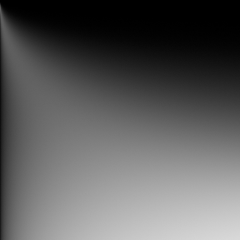 $E_{\mathbf{first}}(\omega)$ precomputed into a 2D texture. You could even get away with a LUT as small as 16x16 given how smooth it is.
We'll have to roll up our sleeves to get Fresnel into the equation (pun intended) in a way that isn't at odds with practicality that a realtime system needs. Once we finalize that, we will jump into the work of Turquin who had a pretty interesting hot take on an approach of this flavor (of which Sony's Imageworks people are also proponents of)... He, interestingly, opted in to variably scale the single-scattering BSDF instead of manually developing a secondary term like we just did. And if you'd like to see a "before/after" image, I've got you covered:
 The difference is rather striking at high roughness!
The furnace differential at high roughness is the best argument for approximating multiscattering.