
This is a refurbished version of two of my articles from 2007 in the interest of answering two questions that have been raised on Discord recently, mostly to be used as additional reading / reference for my newer articles.
On the non-linear depth buffer
The way we transform depth in the perspective projection matrix comes off as weird if you've never written a software rasterizer before, especially one modeled around emulating the way actual hardware (ie a GPU) would do it. To address the elephant in the room: no, it's not mandatory. It's just useful, as you'll see in the next few paragraphs.
As you know, one of the fundamental considerations behind any rasterizer is interpolating depth stored at vertices across the surface of the triangle they define for the purposes of hidden surface removal, determining what lies on top of what in the final image. A naive approach would be to simply, and trivially, linearly interpolate it in screen space. The issue with this should be obvious, the triangle being rasterized can have any orientation with respect to the image plane meaning that its projection won't be a mere simple linear scale down unless the triangle lies in a plane that is head-on parallel with the image plane hence the interpolation based on factors derived in screen space will be incorrect. We thus want to find a relation which will allow us to effectively interpolate depth on the triangle in view space because, again, uniform steps in the image plane do not necessarily map to uniform steps in the plane containing the triangle. From the diagram below, the following can be derived:
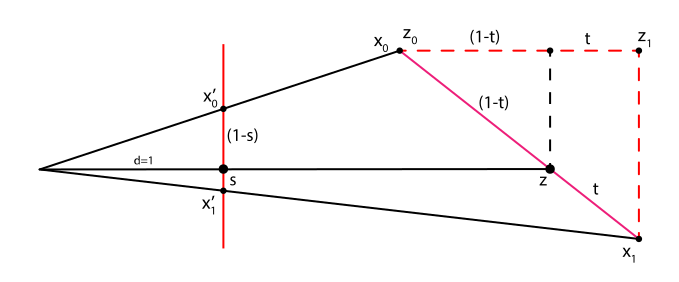
$$\begin{split} z_0 + t(z_1 - z_0) = \frac{x_0^{'}z_0 + t(x_1^{'}z_1 - x_0^{'}z_0)}{x_0^{'} + s(x_1^{'} - x_0^{'})} \iff \frac{x'}{d} = \frac{x}{z} \\ \end{split}$$
A little bit of rearranging gets us $t$ in terms of $s$, our ticket to interpolating in view space:
$$t\left[ z_1 + s(z_0 - z_1) \right] = t\left[ (1-s)z_1 + sz_0 \right] = sz_0$$ $$t = \frac{sz_0}{(1-s)z_1 + sz_0} $$
Plugging it back in causes a healthy number of satisfying cancellations, leaving you with:
$$z = z_0 + \frac{sz_0(z_1 - z_0)}{(1-s)z_1 + sz_0} = \frac{z_0z_1}{(1-s)z_1 + sz_0} $$
You could call it quits here, but the right side yearns to be simplified:
$$z = \frac{z_0z_1}{(1-s)z_1 + sz_0} \Rightarrow \frac{1}{z} = (1-s)\frac{1}{z_0} + s\frac{1}{z_1}$$
Even better, trying to interpolate in the plane of the triangle revealed to us that $1/z$ interpolates linearly in screen space, a fundamental result in rasterization. Hardware likes linear interpolation. This is why we model our depth transform function encoded within the perspective projection matrix as $d(z) = A + B/z$ (following the $z$-divide from the basic linear scale-translate $Az + B$). Depending on graphics API, the range of the function has different limits. In D3D land, by default, depth is mapped from $[n,f]$ to $[0,1]$, to normalized device coordinates. When using single precision floating points, most resolution in this scenario is packed really up-close which makes the rest of the depth range fight for scraps, potentially leading to z-fighting. This is why most of us flip the depth test to the slightly unnatural greater_than (along with a near/far reversal), to enable clean rendering of longer distances.
It is important to note that the non-linear depth is not used for perspective-correct vertex attribute interpolation, as the transform destroys the necessary information. It is mainly used for ordering-related operations, primarily fast hidden surface removal. This allows the GPU to intercept unnecessary computations on geometry which will not be visible on-screen via early-Z checks, avoiding costly perspective-correct attribute interpolation and dispatching pixel shader workloads. Naturally, this also makes shadow mapping faster and simplifies implementation of certain shaders (such as finding edges) because depth discontinuities are trivial to detect.
On texture swizzling
The most common, and easiest to understand, method of "flattening" a 2D array of data is usually to store it row-by-row (row-major) or column-by-column (column-major). Pretty much any texture will have very long rows and columns, so any processing on a local block of texture data (such as bilinear filtering) will mean cache misses and DRAM page breaks.
What we want is to flatten the texture tile-by-tile (eg. 2x2) or even by doing tiles that contain smaller tiles (4x4 tiles containing 2x2 tiles etc). A naive way you may come up with is by using the modulus operator to define blocks, but that is hardly performant. In the diagram, you can see how a row-major texture looks like in memory by drawing lines through the rows and an example of what we'd like to see. Notice that both exhibit a Z-like pattern. That is crucial.

Assumptions made in this section
In all the examples, assume that I am talking about a power-of-2 sized 2D texture with a single channel with 1 byte worth of data unless explicitly stated otherwise. This makes addressing expressions simple and easy to digest. You can extrapolate from the intuition gained to see how it works on more elaborate configurations.
When accessing row-major data, we utilize a stride that helps us navigate between rows as the we $y$ coordinate increases. In the simplest case where each entry is $1$ byte long and rows are not padded for alignment concerns that stride is just the width of the texture, so you'd express it the desired linear address as $y*w + x$. Multiplication of integers is nothing but shifts and adds, so any number of coordinates with well defined layout of rows and slices can be fully linearized as a combination of shifts and adds. In the case of power-of-2 sized textures, it boils down to a single left shift and add. For a 256x256 row-major texture, from the bits of the individual coordinates you can form any address with $\mathrm{y_7y_6y_5y_4y_3y_2y_1y_0x_7x_6x_5x_4x_3x_2x_1x_0}$. After all, it's just the left shifted $y$ coordinate (multiplied by $256$) $\mathrm{y_7y_6y_5y_4y_3y_2y_1y_000000000}$ and the $x$ coordinate $\mathrm{00000000x_7x_6x_5x_4x_3x_2x_1x_0}$ added to it.
The linear address allows the $x$ coordinate to go all the way up to 255 and the $y$ dictates the offset for the row we're targeting. As you've seen, the Z pattern is already there, it's just extremely long. You can shorten that interval by bit twiddling. The simple act of permuting to $\mathrm{y_7y_6y_5y_4y_3y_2y_1x_7x_6x_5x_4x_3x_2x_1y_0x_0}$ creates rows of 2x2 tiles, making $(x,0)$ go $0, 1, 4, 5, 8, 9, 12, 13, 16, 17$... Any number of nested tiles are possible, including the pattern I drew in the diagram above with 2x2 tiles inside of 4x4 tiles. The top-level tile dimensions dictate padding requirements for the texture and thus how much memory will be wasted.
Methods for bit twiddling
How one actually interleaves the necessary coordinate bits to get the final linear address is both tricky and not. In software, it can get quite messy getting this to run fast, usually we utilize tricks with multiplication being just shifts and adds to actually goad the bits into spacing out and then adding them together to form the final address. Adding is often used instead of bitwise OR because there are special addressing modes for addition with two operands on most, if not all, relevant hardware architectures.
GPUs have special dedicated hardware for this as it's nothing but routing circuitry, it can be made extremely fast if the swizzle pattern is hardcoded. x86 CPUs have had "bitwise scatter/gather" instructions for quite a while, called PDEP/PEXT for deposit and extract. Intel has implemented the instruction in hardware since Haswell while AMD was doing it in very latent microcode all the way up to Zen2 (latency of 18, IIRC). Zen3 is the first generation of AMD CPUs with actual proper support for the two instructions, making them feasible and fast. In case you were writing a software rasterizer on your new 5950X for shits and giggles.