
Things worth noting...
A no-op will always be faster than any other op. Hence, while the technique outlined here is ridiculously performant, I don't actually utilize the system in realtime as it is not necessary for most use cases (exceptions being animations). On my end, every static bit of UI is rasterized quickly at load time and again only if DPI changes are detected. That way you can ship light vector graphics data and generate a system specific collection of supersampled rasters that are calibrated for the highest DPI monitor in use.
With the ever-increasing pixel density of modern displays and the less than satisfying didactic coverage of vector graphics, there's been growing interest among my colleagues regarding my hardware-accelerated implementation. In this article, I will attempt to quickly outline a simplified, scanline-based approach I implemented for use with my custom GUI framework and, by extension, Police Line. Modest knowledge of Bezier curves is a prerequisite for the reader, some of which can be acquired in a previous article.
Commercial and academic state of the art
Whenever I mention I wrote a custom, online vector graphics rasterizer, most guess it is based on ideas developed by Loop and Blinn in 2005 or Kerr in 2009. Alas, both approaches require runtime CPU-based precomputation which easily becomes the bottleneck when processing complex vector graphics.

The former triangulates the path vertices on the CPU to generate geometry that represents the filled interior while parametrically solving the partially covered boundary in what is effectively texture space on the GPU. The latter, used in Direct3D 11-based Direct2D, is not entirely dissimilar as it revolves around converging to the path interior through trapezoid tessellation, a costly step performed, once again, on the CPU. Which is to say, both guesses are wrong.
While there have been developments as late as 2019 which propose generalizing 2D patch primitives suitable for GPU processing, they still require a hefty precomputation of whichever paths one desires to rasterize. Managing that doesn't seem particularly enticing given that the resulting speed-up is not necessarily stellar compared to my preferred approach, parallelizing the conventional scanline method. I reckon the most recent paper on the parallelized scanline rasterizers was written by Li et al. in 2016.
The paper, while interesting, has issues. It somewhat tends to hand-wave away important details, implies more complicated mechanisms are at play than in actuality and the supplementary code is fairly bad, even for academics. To add insult to injury, the provided reference implementation is written against the vendor-locked CUDA which is hardly appropriate for a purported solution to a real world problem.
Vector graphics in the game industry
Current commercial landscape is also rather sad, the middleware of choice for AAA studios, Scaleform is notoriously expensive and slow with games such as the latest Spiderman burning up to 8 ms on the UI alone. Microsoft's Direct2D, as outlined by Kerr in 2009, has an expensive CPU-side geometry generation and tessellation step and, as an API, is almost universally hated. With the advent of Direct3D 12, it cannot be used without serious issues and complications that arise from the Direct3D11on12 "translation layer" as it was built on top of the traditional Direct3D 11 API. Once and if you try to combine it with DirectComposition, it pretty much implodes.
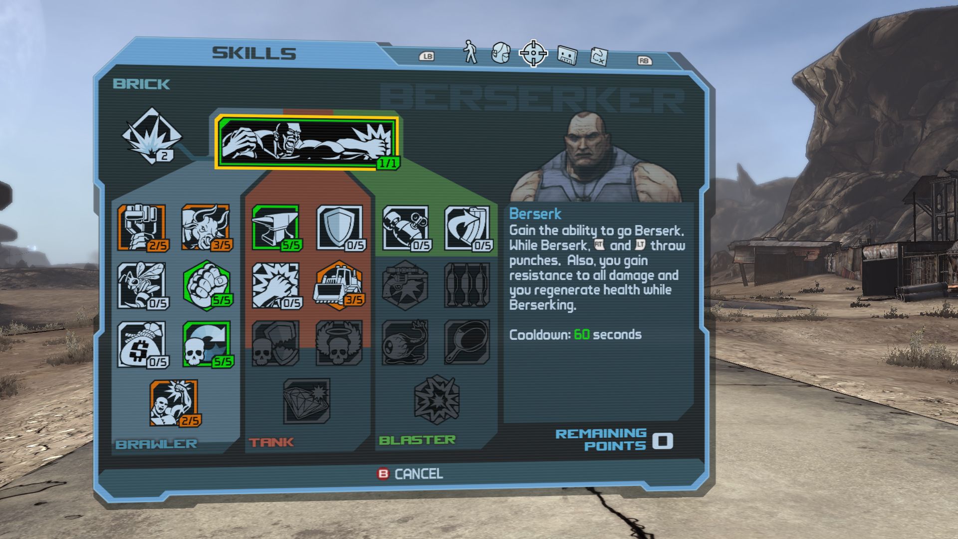 Scaleform in Borderlands
On the other end of the spectrum, offline rasterized UI graphics at multiple resolution "LoDs" seems to be the nominal approach for apps on Apple devices, but also many a game. The latter sometimes just cover the bare minimum (96 dpi) which makes returning to them later a blurry mess.
There are also alternative solutions that are neither here nor there suitable for text rendering, based on signed distance fields. To my knowledge, applying SDFs to text rendering was popularized by Valve back when they were still making games and is actively used today by at least Unreal Engine 4.
Why "vector graphics"?
Early on, vector graphics were tightly coupled with display hardware. As such, they were contrasted against raster graphics displays, thus indicating the freedom of movement of the underlying "electron gun". In conventional raster displays, you had scanlines along which the electron gun moved from left to right, filling every discrete point as it went by according to the video signal. Vector graphics displays on the other hand had the the ability to move the gun's target in any pattern they desired, enabling them to move from point to point to draw a line. By continuously altering the direction, you could also display curves easily. Hence the somewhat counterintuitive name at first glance. It is no accident that we use the term nowadays as it is exact in spirit, original vector graphics displays were resolution independent and scaled nicely. Even the drawing information was formulated as a less advanced version of what we have today.
Today, the first association with modern vector graphics is "Bézier curves" and "text rendering". Like vector graphics were originally introduced for the needs of the US military (analysis of radar data), Bézier curves at the core of our modern vector graphics were introduced targeting a higher dimension in service of the French automotive industry by two pioneers, Paul de Casteljau of Citroën and Pierre Bézier of Renault. Both were interested in allowing artists to utilize a wonderful new invention called the computer to shape the bodies of future cars in an intuitive way. The world would learn of this in the 1960s and 1970s, most notably at a graphics conference held by the University of Utah in 1972, the home of the Newell teapot.
Parallelizing the scanline
In the conventional, horizontal scanline rasterization method, the idea is to sweep along the raster grid vertically, intersecting with path curves at each iteration and filling in the spans in-between according to the fill rule (even-odd or non-zero) applied to the accumulated winding number wrt any position on said span. Naturally, this requires the intersections to be ordered. For the longest time, this has been impossible to do on the GPU efficiently due to the method's sequential nature and complex, prolonged computations. It's not any one thing we devised in the meantime as much as it is the increased programmability of GPUs that made it possible. Not only are GPU programs now able to be much more expressive, they can also be far longer as instruction count limitations have virtually been removed.
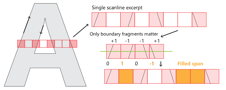
Key observation one needs to make is that the spans between two sequential scanline intersections with curves belonging to the same path all have the same winding number and can be processed as a unit, ie be indirectly scheduled as a hardware-accelerated line draw. More importantly, these spans are completely determined by the two intersections on either end. Specifically, the pixels on the span boundary containing portions of said curves. We shall use OpenGL vernacular and call these boundary/edge fragments as multiple paths may go through the same pixel. It quickly becomes clear that accumulating all those fragments by intersecting all the individual curves with the pixel grid will set the foundation for our rasterization method.
As multiple curves may land onto the same pixel and generate separate boundary fragments, we will also need to merge fragments that intersect curves that belong to the same path as they need to be processed as a unit. As the paths do not necessarily cover every pixel grid line, it would be wrong to run a thread for every grid line. Our parallelization basis for this stage will thus be the individual curves of each path. This may set off a red flag for you. Rightly so, curves that are way too long will intersects thousands of grid lines. As a bake step, you can convert any long path curves to shorter curves as a function of arbitrary heuristics that are up to you and your project's needs.

At this stage, we need to perform numerical root finding to test each relevant grid line against each individual curve dispatched. Most root finding algorithms for "online usage", including the simplest bisection solver, require an interval where samples at the limits have opposing signs. To achieve this, we need to have the curve extremities parked within the axis aligned bounding box of each curve's start and end position to enumerate and process the relevant grid lines without multiple intersections. We need to guarantee convergence for the bisection solver. This means that our inner control points, the tangents, need to be within the said bounding box. In other words, making sure every grid line "within" the bounding box intersects the curve and intersects it once.
We do this by making each curve monotonic, ie only increasing or decreasing wrt either axis. Naturally, we seek the roots of the derivative of each curve to find positions where this trend is broken (ie $t$ where the derivative is $0$ wrt $x$/$y$, indicating a tipping point for the curve). For linear curves (lines), they're already monotonic and we do no work on them. Quadratic curve's derivative is linear, trivial to determine whether it intersects 0. Cubic curve's derivative is quadratic and there is the "famous" solution to find the roots (zero). We collect all these curves and test them against the relevant lines using a bisection solver, this way we can initialize the next iteration from the previous by iterating over the grid lines one-by-one. In the end, we combine the individual $t$s and sort them to get pairs of intersections whose middle will reveal the location of the newly generated boundary fragment.
After accruing the boundary fragments, we need to sort them to actually generate spans between them and separate them by scanline, to allow us to compute the winding number on each of them. We do this by performing stable sorts against the individual coordinates of the boundary fragment as well as the path ID to make sure the "painter's algorithm" is maintained. We also merge all the boundary fragments belonging to the same path ID and pixel. At this point, we can process each merged fragment on its own by running a line through the center and checking for intersections with the constituent subcurves. Depending on the direction of the curve, clockwise yields $1$, counter-clockwise yields $-1$. Once all the merged fragments have this small computation done, we can use a prefix sum (specifically, an exclusive scan) to calculate the winding numbers at each of the possible spans between them. Anywhere where the resulting prefix sum is odd or non-zero (according to whatever fill rule you choose), you render the span between the $i$th and $i+1$th fragment's location, if they're on the same scanline (non-inclusive).

Merged boundary fragments require special attention to actually get to the sample points. By extending vertical and horizontal "rays" (really line-curve tests, rays are merely descriptive) and counting crossings, we determine whether any of the MSAA sample points is covered or not (same deal, $0$ or $2n + 1$). In the end, you manually fill in MSAA coverage information and render all the boundary fragments indirectly as 1x1 lines.
Potential for precomputation and further optimization
The vertical and horizontal line-curve crossing tests for samples are separable and can be precomputed individually for all MSAA samples, stored into lookup tables. The vertical component is solely a function of the individual curve's intersection with the left edge of the boundary pixel. Horizontal is more complicated, but you can arbitrarily approximate each subcurve with lines going through the start, end and $n$ interim points. By deriving the half-plane from each such line, you can precompute and lookup the bitmask of all samples on the relevant side of the line. By repeating this for each line approximation and closing off the top and bottom, a bitwise and will give you the final bitmask. This is linearly combined with the vertical lookup and the main ray to get the final bitmask for the boundary fragment, to be used to fill out MSAA coverage when rendering the 1x1 line representing the fragment.
Fun. Got to go. Bye.