Dark mode is now active. You can revert to light mode at any time by toggling the light bulb button.
Latest posts
Implementing an append buffer in Metal/MSL
Domagoj Pandza on March 3rd, 2018
Programming
Show in single article view

Recently, I had an exchange with a colleague of mine whose background is primarily in conventional graphics APIs with limited compute capabilities, he was complaining about the lack of an intrinsic append buffer in MSL. Certainly not the first time this was brought up to me or somewhere else online. I thought it would make for a good article to show both why an intrinsic one is not necessary and how you can roll your own if you're working with Apple platforms. If you're not familiar with an append buffer in the context of GPGPU, it's a structure geared for queuing entities processed in parallel without in-fighting between threads for a slot, which is to say, it supports temporally unordered access. When it comes down to it, it's really just a simple frontend consisting of a single method which manipulates the underlying buffer and its associated atomic counter.

In HLSL, which is considerably less expressive than MSL, the structure in question is provided intrinsically (AppendStructuredBuffer<T>) as it is impossible to link a counter and a buffer together in a custom generic structure. The buffer which is to be augmented with append functionality needs to have its unordered access view marked as such through the DirectX API on the CPU side. This enables the runtime to procure the necessary atomic counters which are hidden from the user. For us, everything will be a bit more explicit. In the next few paragraphs, you will find out how to hide the atomic counter so the user doesn't have to lug anything around as long as they size the underlying buffer appropriately.

Understanding the limitations of MSL

It's merely a subset

As you're probably familiar, the Metal Shading Language is based on the C++14 specification and a subset of the functionality specified therein, which sounds very impressive and is bound to give people the wrong impression. Before we get to implementing our append_buffer<T>, we need to reiterate on the limitations of MSL so that certain implementation decisions don't feel jarring to those versed in C++, but not necessarily MSL.

Forget about inheritance

It is not possible to extend the functionality of your classes or those provided by the Metal standard library. Naturally, from this follows that virtual specifier (dynamic dispatch) and dynamic_cast are not allowed. Mind you, even if we had some modicum of inheritance, the latter wouldn't work due to the complete lack of runtime type information.

new/delete are not available

As with any other shading language, all persistent allocations are performed through the appropriate APIs on the CPU side and fed into the appropriate shaders running on the GPU, and as usual, both sides need to agree on layout, offsets and bind points. Pointers and references are also limited only to more persistent data locations and require an appropriate address space attribute prefix, one of device/constant/threadgroup/threadgroup_imageblock. Temporaries are passed around solely by value, just like in HLSL. So, if you thought you could pass a struct by constant reference or maybe even move it, nope.

But wait, there is more

Obviously, exceptions are not supported and thus noexcept is meaningless. You can't perform recursive function calls as GPUs are not quite there yet. goto is not available, now if only we could get rid of it in C++20y as well. Storage class specifiers register and thread_local are not available in MSL, former of which was also deprecated in C++11.

Shopping at the atomics store

Atomicity and synchronization operations, memory ordering, atomic data types

The part of the Metal standard library (metal_stdlib) dedicated to dealing with atomics is contained within metal_atomic. Don't worry, you don't have to explicitly include it. There is a myriad of operations available, just like in the C++ standard library itself and intrinsics that come with HLSL. All devices which are certified for Metal 1.0 support relaxed memory ordering and atomic_(u)int. Relaxed memory order makes no guarantees on the ordering of the memory operations as observed from any one thread, but it does guarantee atomicity which is all we need to enable an atomic counter. We'll be using atomic_uint for the counter type and avail ourselves of a read-modify-write operation to increment the counter in one whole swoop, returning the previous value of the atomic data (to index into the underlying buffer). The specific overload is effectively the same as the one in the C++ standard library:

template<typename T> // For atomic integers, atomic<T>::OperandType == T
T atomic_fetch_key_explicit(device atomic<T>* object, atomic<T>::OperandType operand, memory_order order);

// Or more to the point, for low-tier atomics and T is uint:
uint atomic_fetch_key_explicit(device atomic_uint* object, uint operand, memory_order order);

This function is all we need to enable an append buffer on any Metal 1.0 device, going all the way back to an iPhone 5S should that matter to your project. I might cover atomics in general in a future article as I've seen a lot of confusion online regarding why they're needed and how they're used (especially when). For now, let's proceed to write the append buffer implementation.

Putting it all together

With a few considerations

We've got to address the elephant in the room... Sourcing the counter as it needs to have persistent storage to be of any use. In a lesser system, we'd have to lug around at least \(n + 1\) buffers around where the extra one is storing \(n\) counters, one for each append buffer. Passing that around would be a chore and just plain ugly. Remember that allocation is requested by the CPU and resizing on the GPU is not possible, thus we always provide some considerable upper bound which we never expect to reach. So, if we were to tear out sizeof(atomic_uint) from the start of each buffer and use it as the counter, this lets us avoid a lot of boilerplate. Actually, we push up the start of the actual buffer to 16, which is the safest alignment:

template<typename T>
struct append_buffer {

    append_buffer(device T* underlying_buffer) {

        auto untyped_underlying_buffer = reinterpret_cast<device char*>(underlying_buffer);
        _counter = reinterpret_cast<device atomic_uint*>(untyped_underlying_buffer);
        _underlying_buffer = reinterpret_cast<device T*>(untyped_underlying_buffer + 16);

    }

    auto append(T t) {
        auto index_before_increment = atomic_fetch_add_explicit(_counter, 1, memory_order_relaxed);
        _underlying_buffer[index_before_increment] = t;
    }

private:
    device atomic_uint* _counter;
    device T* _underlying_buffer;

};

From here, we can use it in a compute kernel. Every buffer that we bind on a compute command encoder is passed to the compute kernel entrypoint as an argument. I prefer to provide an overarching struct which I consider the compute kernel, which is really "the way it's meant to be played" and refreshing after years of global constant buffers. This helps me consolidate shared data without passing it around a bunch of free functions.

struct compute_kernel {
    
    compute_kernel(uint2 thread_id, device element* elements_buffer) 
    : _thread_id(thread_id), _elements_append_buffer(elements_buffer) {}

    auto execute() -> void;

private:
    uint2 _thread_id;
    append_structured_buffer<element> _elements_append_buffer;

};

auto compute_kernel::execute() -> void {

    // ...
    _elements_append_buffer.append(...);
    // ...

}

kernel auto compute_kernel_entrypoint(

    uint2               thread_id           [[thread_position_in_grid]], 
    device element*     elements_buffer     [[buffer(0)]], 

) -> void {
    
    compute_kernel compute_kernel_instance { thread_id, elements_buffer };
    compute_kernel_instance.execute();

}

Regarding the allocation request for a buffer on the CPU side via Metal API, it's fairly straightforward:

id<MTLDevice> _device;
NSUInteger bufferLength = sizeof(element) * elementCountWithAReasonableMargin;
[_device newBufferWithLength:bufferLength options:MTLResourceStorageModePrivate];

A simple "consume" buffer

To be used in conjunction

For the sake of completeness, the following snippet also describes a very simple "consume" buffer, quotes required as it isn't quite what the HLSL counterpart has in mind, which I find quite useless. It's simply a layer above the underlying buffer which can decode the utilized count of the buffer which can then be used to limit threads from accessing out of bounds:

template<typename T>
struct consume_buffer {

    consume_buffer(constant T* underlying_buffer) {

        auto untyped_underlying_buffer = reinterpret_cast<constant char*>(underlying_buffer);
        _counter = reinterpret_cast<constant uint*>(untyped_underlying_buffer);
        _underlying_buffer = reinterpret_cast<constant T*>(untyped_underlying_buffer + 16);

    }

    auto get_count() {
        return *_counter;
    }

    auto operator[](uint i) {
        return _underlying_buffer[i];
    }

private:
    constant uint* _counter;
    constant T* _underlying_buffer;

};

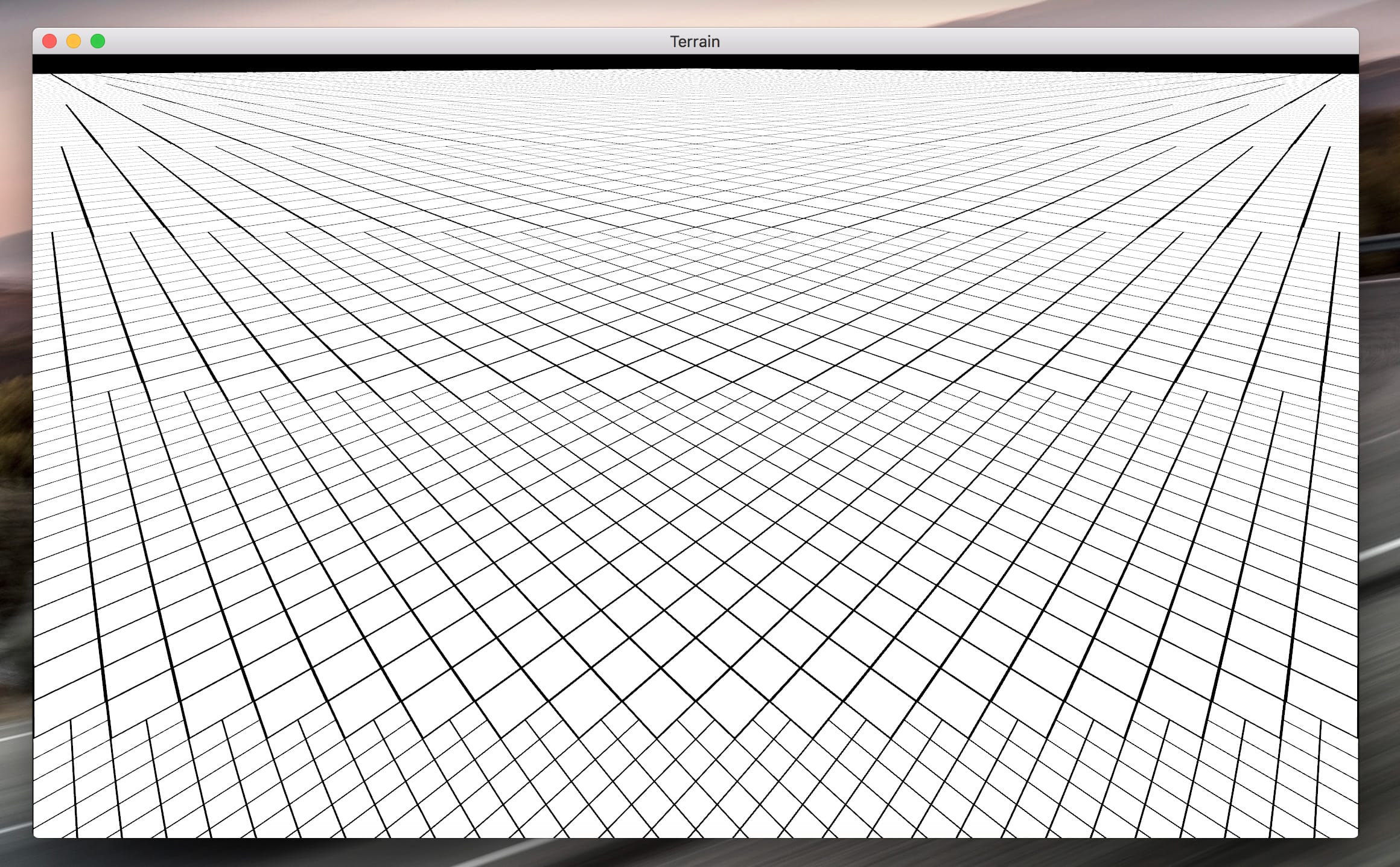
I used a similar setup when I was working on the port of my adaptive terrain solution for Apple platforms for numerous stages which were computed in the geometry shader. You can see the region subdivision stage below.
Until next time.

Vector graphics, scanlines and the highly programmable GPU
Domagoj Pandza on January 26th, 2018
Computer Graphics
Show in single article view

Things worth noting...

A no-op will always be faster than any other op. Hence, while the technique outlined here is ridiculously performant, I don't actually utilize the system in realtime as it is not necessary for most use cases (exceptions being animations). On my end, every static bit of UI is rasterized quickly at load time and again only if DPI changes are detected. That way you can ship light vector graphics data and generate a system specific collection of supersampled rasters that are calibrated for the highest DPI monitor in use.

With the ever-increasing pixel density of modern displays and the less than satisfying didactic coverage of vector graphics, there's been growing interest among my colleagues regarding my hardware-accelerated implementation. In this article, I will attempt to quickly outline a simplified, scanline-based approach I implemented for use with my custom GUI framework and, by extension, Police Line. Modest knowledge of Bezier curves is a prerequisite for the reader, some of which can be acquired in a previous article.

Commercial and academic state of the art

In other words, why bother?

Whenever I mention I wrote a custom, online vector graphics rasterizer, most guess it is based on ideas developed by Loop and Blinn in 2005 or Kerr in 2009. Alas, both approaches require runtime CPU-based precomputation which easily becomes the bottleneck when processing complex vector graphics.

The former triangulates the path vertices on the CPU to generate geometry that represents the filled interior while parametrically solving the partially covered boundary in what is effectively texture space on the GPU. The latter, used in Direct3D 11-based Direct2D, is not entirely dissimilar as it revolves around converging to the path interior through trapezoid tessellation, a costly step performed, once again, on the CPU. Which is to say, both guesses are wrong.

While there have been developments as late as 2019 which propose generalizing 2D patch primitives suitable for GPU processing, they still require a hefty precomputation of whichever paths one desires to rasterize. Managing that doesn't seem particularly enticing given that the resulting speed-up is not necessarily stellar compared to my preferred approach, parallelizing the conventional scanline method. I reckon the most recent paper on the parallelized scanline rasterizers was written by Li et al. in 2016.

The paper, while interesting, has issues. It somewhat tends to hand-wave away important details, implies more complicated mechanisms are at play than in actuality and the supplementary code is fairly bad, even for academics. To add insult to injury, the provided reference implementation is written against the vendor-locked CUDA which is hardly appropriate for a purported solution to a real world problem.

Vector graphics in the game industry

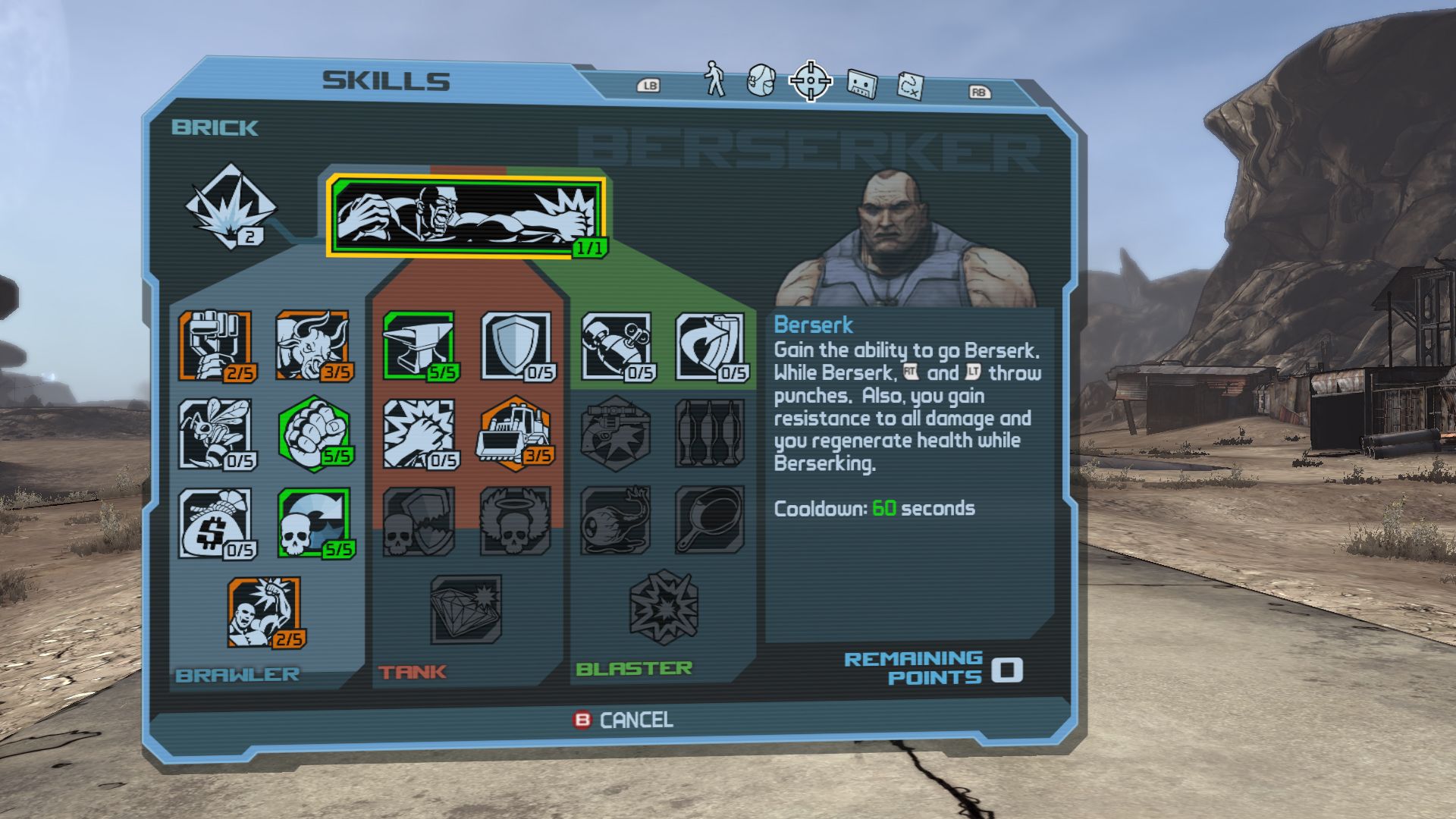
Current commercial landscape is also rather sad, the middleware of choice for AAA studios, Scaleform is notoriously expensive and slow with games such as the latest Spiderman burning up to 8 ms on the UI alone. Microsoft's Direct2D, as outlined by Kerr in 2009, has an expensive CPU-side geometry generation and tessellation step and, as an API, is almost universally hated. With the advent of Direct3D 12, it cannot be used without serious issues and complications that arise from the Direct3D11on12 "translation layer" as it was built on top of the traditional Direct3D 11 API. Once and if you try to combine it with DirectComposition, it pretty much implodes.

Scaleform in Borderlands

On the other end of the spectrum, offline rasterized UI graphics at multiple resolution "LoDs" seems to be the nominal approach for apps on Apple devices, but also many a game. The latter sometimes just cover the bare minimum (96 dpi) which makes returning to them later a blurry mess.

There are also alternative solutions that are neither here nor there suitable for text rendering, based on signed distance fields. To my knowledge, applying SDFs to text rendering was popularized by Valve back when they were still making games and is actively used today by at least Unreal Engine 4.

Why "vector graphics"?

Early on, vector graphics were tightly coupled with display hardware. As such, they were contrasted against raster graphics displays, thus indicating the freedom of movement of the underlying "electron gun". In conventional raster displays, you had scanlines along which the electron gun moved from left to right, filling every discrete point as it went by according to the video signal. Vector graphics displays on the other hand had the the ability to move the gun's target in any pattern they desired, enabling them to move from point to point to draw a line. By continuously altering the direction, you could also display curves easily. Hence the somewhat counterintuitive name at first glance. It is no accident that we use the term nowadays as it is exact in spirit, original vector graphics displays were resolution independent and scaled nicely. Even the drawing information was formulated as a less advanced version of what we have today.

Today, the first association with modern vector graphics is "Bézier curves" and "text rendering". Like vector graphics were originally introduced for the needs of the US military (analysis of radar data), Bézier curves at the core of our modern vector graphics were introduced targeting a higher dimension in service of the French automotive industry by two pioneers, Paul de Casteljau of Citroën and Pierre Bézier of Renault. Both were interested in allowing artists to utilize a wonderful new invention called the computer to shape the bodies of future cars in an intuitive way. The world would learn of this in the 1960s and 1970s, most notably at a graphics conference held by the University of Utah in 1972, the home of the Newell teapot.

Parallelizing the scanline

Implicitly. Bring your scissors.

In the conventional, horizontal scanline rasterization method, the idea is to sweep along the raster grid vertically, intersecting with path curves at each iteration and filling in the spans in-between according to the fill rule (even-odd or non-zero) applied to the accumulated winding number wrt any position on said span. Naturally, this requires the intersections to be ordered. For the longest time, this has been impossible to do on the GPU efficiently due to the method's sequential nature and complex, prolonged computations. It's not any one thing we devised in the meantime as much as it is the increased programmability of GPUs that made it possible. Not only are GPU programs now able to be much more expressive, they can also be far longer as instruction count limitations have virtually been removed.

Key observation one needs to make is that the spans between two sequential scanline intersections with curves belonging to the same path all have the same winding number and can be processed as a unit, ie be indirectly scheduled as a hardware-accelerated line draw. More importantly, these spans are completely determined by the two intersections on either end. Specifically, the pixels on the span boundary containing portions of said curves. We shall use OpenGL vernacular and call these boundary/edge fragments as multiple paths may go through the same pixel. It quickly becomes clear that accumulating all those fragments by intersecting all the individual curves with the pixel grid will set the foundation for our rasterization method.

As multiple curves may land onto the same pixel and generate separate boundary fragments, we will also need to merge fragments that intersect curves that belong to the same path as they need to be processed as a unit. As the paths do not necessarily cover every pixel grid line, it would be wrong to run a thread for every grid line. Our parallelization basis for this stage will thus be the individual curves of each path. This may set off a red flag for you. Rightly so, curves that are way too long will intersects thousands of grid lines. As a bake step, you can convert any long path curves to shorter curves as a function of arbitrary heuristics that are up to you and your project's needs.

At this stage, we need to perform numerical root finding to test each relevant grid line against each individual curve dispatched. Most root finding algorithms for "online usage", including the simplest bisection solver, require an interval where samples at the limits have opposing signs. To achieve this, we need to have the curve extremities parked within the axis aligned bounding box of each curve's start and end position to enumerate and process the relevant grid lines without multiple intersections. We need to guarantee convergence for the bisection solver. This means that our inner control points, the tangents, need to be within the said bounding box. In other words, making sure every grid line "within" the bounding box intersects the curve and intersects it once.

We do this by making each curve monotonic, ie only increasing or decreasing wrt either axis. Naturally, we seek the roots of the derivative of each curve to find positions where this trend is broken (ie $t$ where the derivative is $0$ wrt $x$/$y$, indicating a tipping point for the curve). For linear curves (lines), they're already monotonic and we do no work on them. Quadratic curve's derivative is linear, trivial to determine whether it intersects 0. Cubic curve's derivative is quadratic and there is the "famous" solution to find the roots (zero). We collect all these curves and test them against the relevant lines using a bisection solver, this way we can initialize the next iteration from the previous by iterating over the grid lines one-by-one. In the end, we combine the individual $t$s and sort them to get pairs of intersections whose middle will reveal the location of the newly generated boundary fragment.

After accruing the boundary fragments, we need to sort them to actually generate spans between them and separate them by scanline, to allow us to compute the winding number on each of them. We do this by performing stable sorts against the individual coordinates of the boundary fragment as well as the path ID to make sure the "painter's algorithm" is maintained. We also merge all the boundary fragments belonging to the same path ID and pixel. At this point, we can process each merged fragment on its own by running a line through the center and checking for intersections with the constituent subcurves. Depending on the direction of the curve, clockwise yields $1$, counter-clockwise yields $-1$. Once all the merged fragments have this small computation done, we can use a prefix sum (specifically, an exclusive scan) to calculate the winding numbers at each of the possible spans between them. Anywhere where the resulting prefix sum is odd or non-zero (according to whatever fill rule you choose), you render the span between the $i$th and $i+1$th fragment's location, if they're on the same scanline (non-inclusive).

Merged boundary fragments require special attention to actually get to the sample points. By extending vertical and horizontal "rays" (really line-curve tests, rays are merely descriptive) and counting crossings, we determine whether any of the MSAA sample points is covered or not (same deal, $0$ or $2n + 1$). In the end, you manually fill in MSAA coverage information and render all the boundary fragments indirectly as 1x1 lines.

Potential for precomputation and further optimization

The vertical and horizontal line-curve crossing tests for samples are separable and can be precomputed individually for all MSAA samples, stored into lookup tables. The vertical component is solely a function of the individual curve's intersection with the left edge of the boundary pixel. Horizontal is more complicated, but you can arbitrarily approximate each subcurve with lines going through the start, end and $n$ interim points. By deriving the half-plane from each such line, you can precompute and lookup the bitmask of all samples on the relevant side of the line. By repeating this for each line approximation and closing off the top and bottom, a bitwise and will give you the final bitmask. This is linearly combined with the vertical lookup and the main ray to get the final bitmask for the boundary fragment, to be used to fill out MSAA coverage when rendering the 1x1 line representing the fragment.

Fun. Got to go. Bye.

Generalizing the van der Corput sequence to two dimensions
Domagoj Pandza on January 14th, 2018
Mathematics
Show in single article view

In a previous article, we discussed how one can arrive at the van der Corput sequence, which is a low discrepancy sequence defined on the unit interval. While it is interesting on its own, generalizing it to higher dimensions is where it becomes useful in computer graphics applications. Applications where we often desire well distributed random samples that, for example, cover a domain uniformly for the purposes of estimating integrals. There is the standard approach of using pseudorandom number generators which have the unfortunate result of clumping samples together and poorly estimate integrals at low sample counts. As we've shown in the previous article, even though the van der Corput sequence is completely deterministic and predictable, it has the visual appearance of randomness (difficult to observe patterns) and has a very low upper bound on discrepancy meaning it is very near to being uniformly distributed.

Adding another dimension

Generalizing to 2D

The most trivial way to generalize the van der Corput sequence is to sample a separate van der Corput sequence for each axis. Obviously, they cannot be the same elements and they cannot be elements derived from the same sequence at some procedural offset as that creates a link between the two, an observable pattern. The only remaining thing to generalize then is the granularity at which the reflection around the radix point is performed, which in the vanilla case is derived from base \(2\). If we make it \(b\), the expression for our generalized van der Corput sequence becomes:

$$ \left( \sum_{k = 0}^{\log_b(i)+1}{d_k^b(i)b^{-k-1}} \right)_{i\in\mathbf{N}} $$

We desire to specify a sequence which constructs pairs or points, based on the generalized van der Corput sequence with an arbitrary base. We can specify one such sequence which maps from \(\mathbf{N}\) to \(\mathbf{R}^2\):

$$ \left( \left( \sum_{k = 0}^{\log_{b_0}(i)+1}{d_k^{b_0}(i)b_0^{-k-1}}, \sum_{k = 0}^{\log_{b_1}(i)+1}{d_k^{b_1}(i)b_1^{-k-1}} \right) \right)_{i,b_0,b_1\in\mathbf{N}} $$

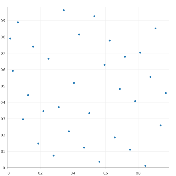
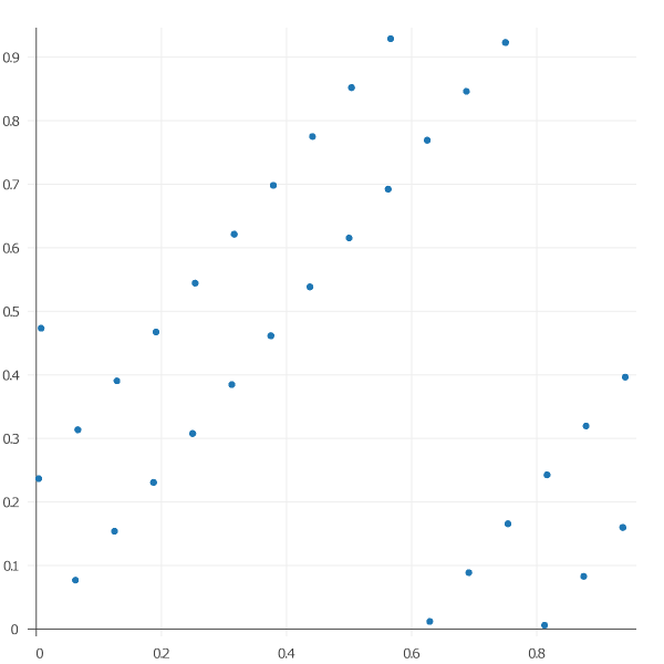
Now, let's take it for a spin. We'll leave \(b_0\) at "native" \(2\) and set \(b_1\) to \(3\) because \(1\) is invalid. Here's \(32\) points with that configuration, we'll also prune the first element of the sequence, \((0,0)\) by means of a constant offset into the sequence, because it's not very useful:

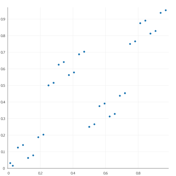
Taking the base pair \((2, 3)\) was the obvious and easiest first choice. Obviously, other choices work too with varying success. The larger the bases involved, the fewer digits are required to describe any given natural number. Let's take a look at what happens when we choose powers of \(2\) for the bases, by drawing 32 samples from a \((2, 4)\) sequence. You might guess this is a poor idea.

As you might imagine, choosing \(b_1 = 4\) is very much like using a constant offset into identical sequences, they become correlated and patterns emerge. Thus, we require the bases to be coprime, in other words, the only positive integer that divides both of them is \(1\). Anything else is equivalent to using the same base sequence with some offset. So, let's try a mutually prime pair, like \((4,3)\):

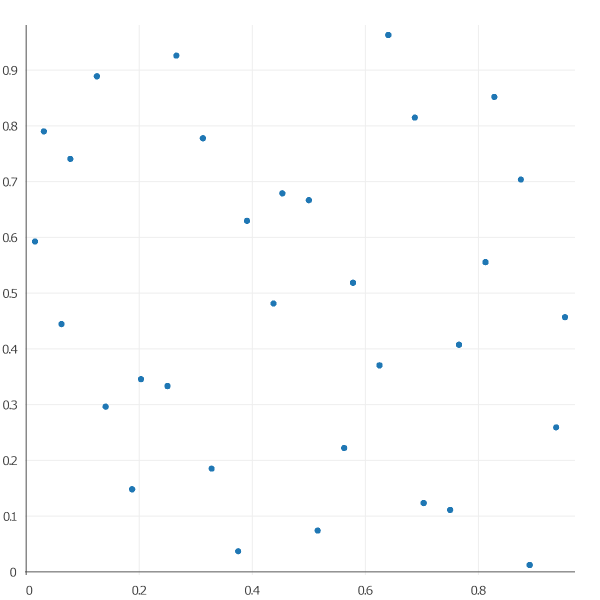
But even coprime bases will result in observable correlation once you get into the double digit bases such as \((16,13)\), as you can see below. Unlike the previous case, though, it is possible to avoid these issues but skipping a number of elements in the sequence depending on the bases used, as well as techniques involving scrambling or outright leaping.

But really, keeping the bases coprime and low is the best option for most applications. The most commonly used bases are \((2,3)\), although I suspect most people use these due to appealing to authority, rather than understanding the issues involved. This type of sequence is called the Halton sequence, after the gentleman who proposed it in 1964.