A brief history with some spicy drama

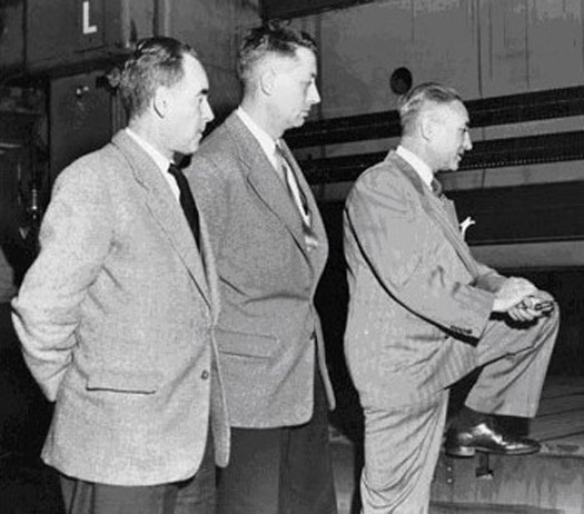
Bézier is the feller in the middle.

It was indeed Pierre Bézier who first popularized the application of these curves in computer aided design of automotive bodies while working at Renault in the 1960s. Renault at the time didn't have a gag order on research disclosure, which allowed Bézier to get his name attached to them under the "I was first to say I was first here" doctrine.

The primary historical reference is still the one by Bézier from a conference at the University of Utah in 1972, a university now famous in the computer graphics community for many contributions to the field and the home of the Newell teapot.

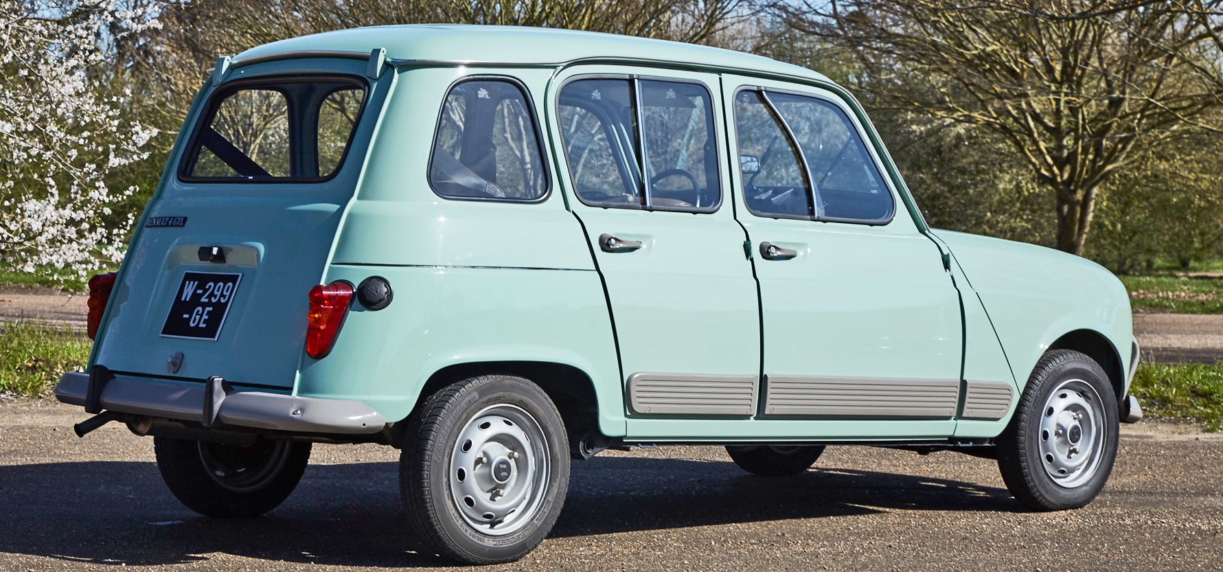
Brought to you by curvy curves.

The thing is... There was another gentleman going by the name of Paul de Casteljau who also worked at a French automotive giant, Citroën... Who claimed to have developed the same curves for the same purpose in the late 1950s, but was barred from publishing his research. Ouch. Now, I am not saying de Casteljau didn't like Bézier much, but he didn't like him. Probably because Bézier patented his life's work. Much like the feud between Newton and Leibniz, a lot of sparks flew here. By the time this was public knowledge, the industry had pretty much associated Bézier with the curves...

The consolation prize attributed to de Casteljau was the "algorithm" used for evaluating the curves. The "algorithm" is merely an unavoidable fact of life, a trivial transformation of the curve equation, and Bézier had to have derived it himself to derive an actionable mathematical basis. While it stings, it's just yet another example of Stigler's law of eponymy, itself a necessity due to the proven possibility of multiple discovery.

Connecting the dots

To achieve anything of note in life, one needs a motivation. One look at curves in analytic geometry and you can see just how much a hassle it is to control/shape the curves intuitively, making our motivation rather clear; finding a way to intuitively control curves as a function of their endpoints and the associated tangent vectors which can be transformed into control points of some sort.

Linear Bézier curve

Our starting point is fundamental analytic geometry and the first construct introduced in analytic geometry is the line. It is fairly trivial to recover a line that goes through two points:

It can be quickly rearranged into a parametric equation as a function of $t$ limited on a $[0,1]$ range:

In the context of Bézier curves, this is the linear Bézier curve. Stating the obvious, but it is also the expression for linear interpolation.

Quadratic Bézier curve

Don't get spoiled by the triviality exhibited so far as we're going up a degree. The first proper curve one is introduced to is usually the ubiquitous parabola. Specified in slope-intercept form, it's $y = a_2t^2 + a_1t + a_0$. If you transform it a bit, you get $y = (a_2t + a_1)t + a_0 = a(t)t + a_0$. The parabola is, thus, what happens when you linearly vary the highest degree coefficient of a line (the directional one). Thus, the derivative of a parabola is a line. As a parabola exhibits mirror-symmetry, the derivative at two points on opposite sides will be mirrored (going up, going down). In other words, they are correlated and it is possible to express the tangents as a function of the end points and a third, shared control point.

While we expressed a linear Bézier curve rather intuitively and satisfyingly by linearly interpolating its end points, the quadratic Bézier curve will not yield as easily. It does have a satisfying analogue; we can elegantly express its derivative at any point as a linear interpolation between the two endpoint "velocity vectors" or tangents specified, due to reasons elaborated in the previous paragraph, as $\mathbf{T_0} = \mathbf{P_1} - \mathbf{P_0}$ and $\mathbf{T_1} = \mathbf{P_2} - \mathbf{P_1}$:

If you're not sure why there is a factor of $1/2$ in there, it follows from the fact that the derivative of $x^2$ is $2x$. You have to be mindful of the established rules while we're playing this constructive game. By integrating this and solving for the $c$ (you're right, it's $\mathbf{P}_0$), we recover $\mathbf{P}(t)$:

And just like that, we have the quadratic Bézier curve. If you swap in the control points, you have a very easy way of evaluating quadratic curves which is sufficient for specifying glyphs of fonts for text rendering. However, to go beyond, one can perform mental gymnastics like the ones we did here. Or we can look for some pattern here. As we have derived the linear Bézier curve as a simple linear interpolation of the end points and the quadratic Bézier curve by noticing its derivative can be expressed in terms of a linear interpolation of the velocity vectors... It just might lead to some generalization if we unroll everything and try to rearrange a bit:

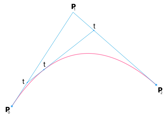
Well, it's a triple linear interpolation, isn't it? The result is the linear interpolation of the linear interpolation between the first end point and the control point and the linear interpolation of the control point and second end point. Given that is true, it can be trivially rephrased as:

That is beginning to look an awful lot like the algorithm attributed to de Casteljau. And this is one way of arriving at it that I find particularly intuitive. Rearrangement following the result of an intuitive base assumption. You don't go trying "well, maybe we do triple interpolation" without any real argument to do so. Especially because you need to understand how $t$ plays into it. I mean, you can, but stumbling onto it is not a good look. At least, as far as I'm concerned.

Cubic Bézier curve

If a linear Bézier curve can be represented with a single linear interpolation, a quadratic with three... Well, now we have a leg to stand on and posit that a cubic could be represented with six, using the same tree-like approach! It also stands to reason there will be two control points aiding the two end points:

Which can be further rearranged and expressed in terms of the points as:

Those are some mad binomial expansion vibes. Or, if you have a stronger background in mathematics to contrast against, Bernstein polynomials come to mind. But notice how we didn't need Bernstein polynomials to define the curves underlying all of modern vector graphics. For completeness and generalization, we are going to go there, though.

Deriving Bernstein polynomials to take us the rest of the way

From the result of the proof, it becomes obvious that the mathematical foundation of the binomial distribution can be transformed into basis functions which, when linearly combined with coefficients, are capable of approximating any well-behaved function. Bernstein polynomials can therefore be defined implicitly as:

$n$-choose-$k$ may obscure the fact that the following is true:

Obviously, it works for the linear case as well:

As it does for the cubic, the quartic and the $n$-th degree curve case. If you feel like it, work them out. You don't really need more than quadratic and cubic curves in practice, in the field of vector graphics at least.

In a previous article, we showed how one can arrive at quaternions. They are exceptional at handling rotations in three-dimensional Euclidean space, providing an efficient and elegant representation free of mapping singularities. However, they're not very useful when it comes to handling other affine transformations, most notably translation and scaling. Scaling can be forgiven, but translation is crucial to enabling rigid transformations and applications in many fields from robotics to computer animation.

Bootstrapping translations

We already showed that the only way to procure a "proper" rotation with quaternions (the conical transformation you're used to from linear algebra) is to compute $\mathbf{p}' = r\mathbf{p}r^*$. Thus, it is reasonable to assume that our translation transformation should assume the same format in the interest of composition with rotations. In other words, we expect $\mathbf{p}' = t\mathbf{p}t^*$. We can also assume a double translation should occur just like with rotations. However, regular quaternion multiplication is unable to perform such a feat without augmentation facilitated by changing/adding rules.

Let us focus on the $t\mathbf{p}$ part of the transform. We represent the position as a pure quaternion (zero scalar component) and assume it makes some sense to have the translation quaternion be one as well, at least for now. We need to augment quaternion multiplication in some manner to enable the translation transformation. To see what we're working with, let's lay it out:

Obviously, this is far from the desired outcome. One way we can try to move in the right direction is to add a real scalar component to both quaternions, of value $1$:

We could live with a constant scalar part of $1$, but that last term is expectedly just pushing our original problem deeper. However, given that it is a product of our imaginary vector components, if we were to augment them with an indeterminate, say, $\omega$... We could then posit that $\omega^2 = 0$. You might see where I am going with this:

It certainly worked out, but we now need to figure out the implications of introducing the indeterminate $\omega$ into the mix. We do notice that our result is attached to it, reminiscent of the way the imaginary component of a complex number is attached to the indeterminate $i$. Our next goal, in the interest of eventually ensuring proper composition, is to complete the transform. Thus, we need to ensure $tpt^*$ doesn't fail us:

Well, that fell apart quickly. It would appear that the conjugate here doesn't behave in the usual way. It might be prudent for us to come to terms that we're no longer dealing with regular quaternions. To test this theory, we will use a non-trivial case of rotations, but this time performed on our generalized position quaternion (to not break emerging compatibility with translation):

A few things of note are happening here. In the case of rotation, we desire to multiply $r$ with $p$, hence we don't attach $\omega$ to $r$ in order for them not to annihilate. Notice the part of the equation before we apply the conjugate, $(r + \omega r\mathbf{p})$. We appear to be dealing with two quaternions. One that is free and the other which is attached to $\omega$. This leads us to posit that the initially assumed scalar component in the position and translation quaternions was and is actually a quaternion itself, a real quaternion (no imaginary vector component). For lack of a better term right now, we'll call these $\Omega$-quaternions, generically specified as $Q = q + \omega q_{\omega}$. One other thing that we may hazard a guess towards from our experience so far is that any properly transformed quaternion is going to have a free component consisting of a real quaternion valued $1$ and the useful result encoded in the $\omega$-component.

Furthermore, since we're talking about two quaternions, we've been going about conjugation all wrong. It stands to reason that $Q^* = q^* + \omega q_{\omega}^*$. Applying this to our original translation transform attempt, we get:

It might seem like we're back to square one, but we just have to keep molding it to meet our goals. Notice that we can conjugate the $\Omega$-quaternion as before, then conjugate its constituent regular quaternions! This would result in the desired double translation by avoiding inversion while still ensuring rotation gets inverted (as it isn't affected by $\Omega$-quaternion conjugation). To differentiate $\Omega$-quaternion conjugation from regular conjugation, we use an overline. For example, the conjugate of $Q$ is then $\overline{Q}$ and the combined conjugate of $Q$ and its constituent quaternions $(q,q_{\omega})$ is thus $\overline{Q^*} = \overline{Q}^*$. While you're working out the simple proof for that on your own, you might also want to prove that $\overline{(Q_1Q_2)^*} = \overline{Q_2^*}\space\overline{Q_1^*}$. Incorporating these changes, we get:

We're almost ready to combine a rotation and a translation into a rigid transformation, and compute its conjugate. However, to verify the properties of rigid transformations, we will have to generalize the notion of the quaternion norm, usually computed a as $||q|| = \sqrt{qq^*}$. So, we compute:

At this point, we need to take a squared root while being considerate of $\omega$. To this end, we rephrase the problem generically: $(a + \omega b)^2 = a^2 + \omega 2ab = c + \omega d$. From this, it follows trivially that $a = \sqrt{c}$ and $b = d / \sqrt{4c}$. Notice that when the constituent quaternions are real, this looks a lot like something that is kin to complex numbers. We'll cover this in the next section. Armed with these new relations, we conclude:

We now know that the only way to have a unit $\Omega$-quaternion is for the inner product of its constituent quaternions to resolve to $0$. Vanilla rotation is encoded with unit quaternions and has a zero quaternion in the omega component when extended to $\Omega$-quaternions as it performs rotation directly through vanilla multiplication. Thus, the inner product is $0$ and it remains unit here as well. On the other hand, $\Omega$-quaternions encoding translation are composed of a real and pure quaternion which results in their inner product being $0$ as well, making the $\Omega$-quaternion unit if and only if the real quaternion is valued $1$. A fundamental property of normed division algebras is $||qp|| = ||q||||p||$ and this extends to $\Omega$-quaternion, allowing us to surmise the composition of rotation and translation will be a unit $\Omega$-quaternion. We now compute the composition $TR$:

Its conjugate $(TR)^* = R^*T^*$ is given by $\hat{r}^* - \omega\hat{r}^*\mathbf{t}$ which allows us to compute the norm and confirm that it is indeed unit:

Finally, we work out a rigid transformation $(TR)P\overline{(TR)^*}$ of a point $P$ and show mathematically that the point is indeed double rotated then double translated into its transformed position:

And there you have it! A rotation followed by a translation, stored in the omega component of our $\Omega$-quaternion. Historically, this result was first recorded in a journal by one Wiliam Kingdon Clifford in 1873. He based his work on Hamilton's quaternions, meaning he also adopted a lot of his preconceptions, including the iffy notion of dividing vectors which was discarded in modern mathematics, but is pervasive in the paper. He originally named the indeterminate $\omega$ which we've used in our derivation here as a nod to him. In his self-proclaimed "preliminary sketch", Clifford named his precursor "biquaternions". This work would later be picked up by Eduard Study who moved them in the direction of what would eventually become known as a dual quaternions. Our $\Omega$-quaternions are dual quaternions. Like us, Study was interested in applying this construct for rigid transformations. In modern times $\epsilon$ has superseded $\omega$ as the indeterminate element. In the next article, we will extract the notion of dual numbers from our "organically derived" dual quaternions... Which will allow us to consider some interesting properties dual numbers have over their "singular" counterparts.

In this article, we are going to derive the Poisson distribution from the binomial distribution. If you don't know what the binomial distribution is or how to derive it from "scratch", I wrote an introduction to it in a previous article. As for the Poisson distribution, it is, obviously, also a discrete probability distribution whose shtick is quantifying the likelihood of $k$ events happening in some interval provided you know the average number of such events happening in said interval and that each event is independent of the previous ones. In other words, their timing doesn't affect the timing of the subsequent ones.

The boilerplate example is estimating the likelihood of a certain number of floods given statistics accumulated over, say, 10 years. Deviating from the mean on either side will, obviously, adversely affect the likelihood of that number of floods happening during a period of 10 years. All we have to do now is find a way to quantify this concept.

Sending $n$ to $\infty$

As mentioned, we start with the binomial distribution. It tells us the likelihood of having $k$ successes out of $n$ trials. The Poisson distribution tells us the likelihood of $k$ events happening given the average of such events happening during some interval (which is implicit). We know the expected value or the mean of the binomial distribution is equal to $nq$ where n is the number of trials and $q$ is the probability of success of a single trial. The expected value makes sense; the more trials we conduct and the higher the probability of success, the more successes we ought to expect. Thus, another way of expressing the binomial distribution by aliasing $\mu$ as $\lambda$ is:

We don't know what the probability $q$ of any one single trial is, but we know an "overall trend" $\lambda$ which we effectively take to be determined over an $\infty$ number of trials, hence to express the Poisson distribution, we allow the number of trials of $n$ go to infinity:

We start off slow, by moving the constant factors outside:

Notice that the equation can be rewritten as follows:

It is easy to see that the product approaches $1$ when we allow $n$ to tend to infinity, hence:

We rewrite the expression further chasing simplification:

It's immediately obvious that:

The remaining factor might look familiar to the way we define $e$ (taking the limit of $(1 + 1/x)^x$ as $x$ goes to infinity). It's not quite there yet, but it stands to reason we can transform it in a way that it can be expressed as a power of $e$:

Which resolves our distribution to its final form:

While it might not surprise you that the the expected value of this probability distribution is $\lambda$, its variance is also $\lambda$. The moment $e$ crops up in your model, its properties are bound to be interesting.

The motivation for writing this article is twofold. First is completeness, as the binomial distribution is an intuitive starting point for elegantly deriving the Poisson distribution which is a topic of a subsequent article, itself a key ingredient of another article. Second is showing how one can intuitively arrive at the binomial distribution as I run into people, from time to time, who have trouble understanding how exactly it works. While its very name might be intimidating to a beginner, it is based on a very simple and intuitive concept, as you'll see in a moment.

At its core, the binomial distribution is a discrete probability distribution which quantifies the likelihood that given $n$ trials, each with a binary outcome, $k$ of them will be a "success". The simplest example would be a series of coin flips, where the sides can be assigned to be either "success" or "failure".

Heads or tails?

Coins, cards, and dice are the usual suspects when it comes to illustrating concepts in probability theory as they're useful for building intuition. We’ll go with rolling dice just to mix it up a little. Now, here's a question: “If we roll three dice, one by one, what are the odds of getting two sixes?”

Given the probability of success is $1/6$ for each independent roll, only $1$ out of $6$ times is going to result in rolling a six. On that one out of six times, there's only a $1/6$ chance we roll another six, reducing the odds to $1$ out of $36$.

On that $1$ out of $36$ times, there is a considerable chance we will not roll a six as the probability of failure is $5/6$. Thus, our chances decrease slightly to a final $5$ times out of $216$, giving us a roughly $2.3\%$ chance to roll two sixes followed by anything else. Two successes, one failure. Effectively, we computed the probability of a single arrangement of two successes and one failure with $p_s = 1/6$ as:

Notice there are three different ways of getting two successes and a failure, in this case, $\{SSF, SFS, FSS\}$. Our computation only deals with the probability of getting any one of those three possible orderings. Thus the probability of getting two successes and one failure is actually three times higher. To generalize this, let $n$ be the number of trials and $k$ be the number of successes, leaving failures implicitly quantified as $n-k$. We need to know how many ways we can order $k$ successes or $n-k$ failures in $n$ trials. Either will do, so we choose what is explicit, the number of successes. If there are $n$ trials, there is $n!$ ways they can be ordered. When you select the "temporal order" of the first trial, there remain only $n -1$ choices for the second placement and so forth. We're only choosing the placement of $k$ trials, the successes. Hence we need to stop the $n!$ factorial after $k$ "iterations", this is done by dividing it by $(n-k)!$ (write it out if you don't see it). Now we have all the ways we can order $k$ successes in the $n$ trial slots. We're only interested in the unique placements of successes (and thus failures which are implicitly in-between) and given that there are only binary outcomes, some of these unique conceptual orderings of trials will end up aliasing one another once their values are "substituted in", we need to remove those.

Let me show you what I mean. In our trivial example with $n=3$ and $k=2$, there is $3! = 6$ ways to order the trials. There is $3! / (3 - 2)! = 6$ ways to order $2$ successes in the $3$ trials. I will use numbers to indicate temporal ordering of the possible configurations: $\{12, 21, 13, 31, 23, 32 \}$. Notice that ordering successes as $12$ and $21$, $13$ and $31$, as well as $23$ and $32$ results in redundancy. Hence, there is only $3$ unique ways we need to account for. There is $k!$ ways to order $k$ elements, hence we finally divide by $k!$. This brings us to the final equation where $q$ is the probability of success, $k$ is the number of successes and $n$ is the total number of trials:

You might have recognized "n-choose-k" from combinatorics, ways of choosing $k$ successes out of $n$ trials which, while it matches the value, doesn't quite relay the semantics. And if you're wondering about the name, originally, it was Bernoulli who proved that $p_q(k,n)$ we derived in this article is equal to the value of the $k$th term of the polynomial expansion of the binomial power $(q + (1-q))^n$. Careful, don't collapse it. Obviously, it needs to resolve to $1$, we're talking about probabilities.

The distribution itself is inherently discrete which makes defining the cumulative distribution function rather trivial. As the cumulative distribution function tells us the probability that a random variable will end up being less than or equal to $k$, it merely amounts to adding up discrete probabilities up to $k$:

What value to expect?

Like all distributions, we need to discuss the expected value of a random variable drawn from it. In this case, it simply comes down to the average of all the possible values weighted by their probability. You already know how the average is defined from childhood, but if you're wondering why it is defined the way it is, I wrote an article on the subject which gives it an intuitive treatment. As expected, we start with:

Substituting the binomial distribution function for $p(x)$ and $k$ for $x_i$ which can neatly alias the iterator $i$:

From here, we need to simplify. If we could get rid of the leftmost $k$ in a manner which would make the binomial theorem applicable, we'd be able to completely obliterate the sum. To this end, I'd like to point out the following holds:

Given this relationship, we can transform the $k$ out of the sum. Furthermore, if it isn't immediately obvious, $(n-1) - (k-1) = n - k$. Here's the result after our first round of transformations:

As $k - 1$ needs to be larger than or equal to $0$, we set the lower limit of the sum to $1$. To make the binomial theorem applicable, we finalize by extracting a single factor of $q$. Then, we just transform the range to make it more readable by using $j = k - 1$ and $m = n - 1$:

And now we just apply it:

This is my preferred way of arriving at the mean, other approaches feel either circular (depending on the knowledge of the mean in the first place) or are just convoluted. The same approach works for the variance, so I will just tell you it's equal to $nq(1-q)$ should you decide to work it out yourself. Remember, variance is defined as the expected value of the squared deviation of a random variable drawn from the distribution to the mean of the distribution. Simplified, it comes down to:

You already know the squared expected value as it is the mean squared, $(nq)^2$, all you have to do is re-do the dance we did before to calculate the expected value of the squared random variable, meaning you calculate the sum of squares of the possible values weighted by the associated probabilities. Enjoy.

A lot of people use quaternions to represent object orientations and to perform rotations in a dependable way, without actually understanding how they work. This is peculiar as the discovery of quaternions is often cited as perhaps the most documented discovery in the history of mathematics. Unfortunately, Hamilton gave the world a poor first impression because he had trouble understanding quaternions. A decade-long campaign of misinterpretation and confusion later, quaternions $\mathbb{H}$ were whisked away to the plane of oblivion for more than a century, at least as far the mainstream public was concerned. But not before its carcass was picked clean by the likes of Gibbs and Heaviside who independently brought about vector algebra and calculus in the modern sense, among other things.

This article aims to show how quaternions can be derived and why they manage rotations in such an efficient, reliable and elegant manner. It also sets the stage for follow up articles on geometric algebra which will more clearly illustrate the useful properties quaternions have (as they're a subalgebra of it). Not to mention open your eyes to see just how badly one man's confusion in 1843. gave mathematical physics a limp we're yet to get rid of.

A quick rundown of \(\mathbb{C}\)

Complex numbers are the algebraic basis for arriving at quaternions, as their properties motivate the development of quaternions. As you should already know, complex numbers arise when one desires to solve the canonical \(x^2 + 1 = 0\) by defining an indeterminate \(i\) as the solution. Complex numbers have a real and imaginary part, both of which are real numbers. The imaginary part enumerates the indeterminate and when combined with the real part, it forms an algebraic extension of real numbers and enables solutions of polynomials such as the one that motivated the extension. We can write a complex number as:

They may look a bit peculiar to people, but they're as "legit" as real numbers are. Here's a simple example, we will square the expression above and procure yet another complex number:

Much like the set of real numbers \(\mathbb{R}\), \(\mathbb{C}\) is a field which, among other terms, predicates being closed under multiplication. Just like one can plot real numbers on the number line, complex numbers may be plotted in the complex plane which can be visualized as two real number lines setup perpendicular to one another. One plots the real part on the horizontal "axis" and the imaginary part on the vertical one.

Like real numbers, complex numbers define absolute value to coincide with the distance from the origin. Unlike real numbers, though, we have to avail ourselves of some geometric insights to compute the absolute value or modulus. Thus, the absolute value of \(z\) is equal to \(\sqrt{x^2 + y^2}\). While we're here, we may as well introduce the complex conjugate by showing how one can compute the absolute value with its help:

In the complex plane, all complex numbers can be thought of as directed segments from the origin thanks to the associated absolute value / modulus. The behavior or basic addition and subtraction may be reminiscent of what you know of vector algebra, which should give you a clear historical perspective where that came from. However, complex numbers also have interesting geometric interpretations when it comes to multiplying and dividing them. To best illustrate this without actually needing to whip out graphs, we will transform to polar form and further compact it by using Euler's relation:

To transform to polar form, \(r\) is just the absolute value of \(z\), \(|z|\), the distance to the origin. You recover \(\theta\) with \(\tan^{-1}(y/(r+x))\), which is the angle to the horizontal "axis". Now, I want you to observe what happens when you multiply two complex numbers:

Interestingly, the angles from the horizontal axis are being added together while the radii are multiplied together. As we already mentioned, the radius is the absolute value or modulus, the distance to the origin. The fact that the modulus of the product is equal to the product of the two moduli was called the law of the moduli by Hamilton and was one of the requirements when he was searching for quaternions. This rather trivial-looking law is of importance, as we can now talk of a complex number $R$ with $r=1$ which has the ability to rotate $z$ by an angle $\theta$:

This was a profound insight, one sorely known to Hamilton. Keep in mind the commutativity of the complex product, as it is a notable feature courtesy of the commutativity of the addition of real numbers. This result may also encourage one to think about the division of two directed segments:

When two directed segments are parallel (the angle is $0$), the result is the positive ratio of their lengths (and thereby norms). When they're anti-parallel (angle of $\pi$), the exponential degenerates to $e^{i\pi} = \cos\pi + i\sin\pi = -1$ which intuitively signs the ratio of the lengths to be negative. The last option is that they have some general angle of separation, at which point division encodes both angular and length information. In case of unit directed segments, their division can be used to recover the angle between them. Hamilton desperately wanted to generalize this to the third dimension, but given that you have never heard of vector division in this sense in classic vector algebra, you may guess on his success. To be honest, the last two concepts discussed, rotating by a single product and the idea of the quotient of two directed segments, brought the entire ship down through a case of chronic underestimation and shortsightedness. The dogmatic perserverence that the same must hold in three dimensions instead of assuming that they're just special cases of a much more general construct. But more on that later.

Going from \(\mathbb{C}\) to \(\mathbb{H}\)

While the geometric interpretation was never far from Hamilton's mind, the way he arrived at quaternions was purely algebraic. Which incidentally may be one of the problems, because Hamilton and his followers tried to shoehorn the geometric interpretation of complex numbers after the fact without giving proper weight to the whole "adding a new dimension" thing. So, we retread the steps, as promised, but for brevity, we don't make all the wrong turns as part of our derivation.

Hamilton did the obvious expansion of complex theory, he added yet another imaginary part and indeterminate $j$ which squared to $-1$ and was presumed perpendicular to both the real and imaginary axis (when interpreting geometrically). Trouble catches up to us once we try to multiply two generic triplets in this new algebra we're crafting and attempt to see whether it is closed under multiplication like \(\mathbb{C}\) is, but you might guess where this is going:

As expected, a higher grade term emerges and is not going away. To close the algebra, we make the safe assumption $ij = k$ and add $k$ into the mix, which Hamilton himself was dumbfounded by, describing it as a paradox:

Given that we established $ij = -ji$, key being the anticommutative property, we assert $ik = -ki$ and $jk = -kj$ as well. We also hold that $i^2 = j^2 = k^2 = -1$ as we're trying to generalize complex numbers in some way. $ij = k$ imposes $ik = iij = -j$, $jk = -ikk = i$ and $ijk = kk = -1$:

All of this is a pretty big deal, as in the case of triplets there is nothing you can do to close the algebra or, in other words, make $ij$ go away. Once we uncover the exponential form in the next few sections, we will show that the law of moduli holds, along with some information on why it matters. Though, nothing is preventing you from bruteforcing it right now. In case you forgot what the law of moduli was, it's $|q_1||q_2| = |q_1q_2|$. Simple, but extremely potent.

Keeping up with the Hamiltons

Hamilton knew what he wrapped his hands around the day it dawned on him to shift to the fourth dimension. Historical documents suggest he immediately started searching for the geometric interpretation of his discovery, getting basic rotations going by the end of the first day. There were three main notions from complex numbers that he wanted to generalize. The ability of complex numbers to represent directed segments, the ability of complex numbers to rotate those segments via a single complex product and the notion that one could recover useful information akin to the dot product through the concept of vector division. In fact, Hamilton was so obsessed with vector division that he actually defined the quaternion in terms of it: A quaternion is the quotient of two vectors, in the general case.

That obviously isn't the case today, so what happened? A geometric interpretation. In common vernacular, everything is subject to interpretation and there are many views that humans accept as valid even though they're most certainly expressing a subset of the whole truth. Due to Hamilton's heavy bias towards the geometric interpretation of complex numbers and making strong, unsubstantiated assumptions about the behavior of quaternions, he was wrong on many levels. This is a bit disappointing as a physicist should know that many things which are true in two dimensions are outright false or false in the general case in three dimensions or more. One example is the relationship between vector quantities of angular momentum and angular velocity in modern physics. In two dimensions, they share direction. In three dimensions, they can be offset by a considerable angle giving rise to what is sometimes referred to as gyro motion.

Geometric interperation of \(\mathbb{H}\)

The crux of the problem here is that Hamilton failed to recognize the two-dimensional interpretation of complex numbers as the special case, not the norm. Initial surveying of the geometric interpretation of quaternions was done manually, by trying to map out where the result gets placed in three dimensional space (by treating the imaginary part as a directed segment or vector, as positions/directions versus rotations). We will do something a bit different. We recognize how obvious the geometric interpretation of complex numbers becomes in exponential form, so that might be a good start for us. There are multiple ways of arriving at an exponential form, by writing out the series or alternatively going back to Euler's relation with a few tricks up our sleeve. First, verify for yourself that the following statements are all true:

Transform the modulus expression by dividing both sides by $|q|^2$:

Apply the trigonometric identity $\cos^2\theta + \sin^2\theta = 1$ by assuming there exists $\theta$ which satisfies:

As \(\mathbf{\hat{v}}^2 = -1\), the Euler relation holds here as well:

It is immediately visible that a compact exponential form will not trivially reveal how exactly we can achieve rotations through multiplication due to the added dimensionality. Thus we will not make use of Euler's relation here and just proceed in the expanded form. We will attempt, much like Hamilton, to multiply a quaternion representing the rotation \(r\) with a quaternion \(p\) representing the position we're interested in rotating. Hopefully, by expanding, we will determine which part of the rotation quaternion defines the plane of rotation and whether or not an actual proper rotation takes place.

The position quaternion has no scalar component at all, which in this form needs to be eliminated by setting \(\alpha = \pi/2\). And then we just:

It follows that the only way to have a rotated pure quaternion result is iff \( \mathbf{\hat{r}}_v \cdot \mathbf{\hat{p}}_v = 0 \), which is to say that the point needs to be in the rotation plane. This is not very useful. Hamilton was very excited about this, though. He thought he had finally generalized the geometric interpretation of complex numbers to three dimensions with quaternions and some help from the "paradoxical" fourth dimension. This little escapade of ours hasn't been a total bust, though. We now know for sure that \(\mathbf{\hat{r}}_v = \mathbf{\hat{n}}\), it is the rotation plane's normal. Our next step is to explore this further. It is reasonable to expect arbitrary rotations are possible and that the result will be a pure quaternion with its norm preserved. To this end, we must find a way to extrapolate the scalar part from a quaternion. Since we don't have much to go on, removing the scalar part is a good start. This is fairly easy if you remember your conjugation:

Seems rather trivial, but it's useful nonetheless, as we can posit requirements such as that whatever the missing piece of our product, we desire $S(\hat{r}p\hat{q}) = 0$. We also know that proper rotations preserve norm, so $|\hat{r}p\hat{q}| = |p|$. We can constrain $\hat{q}$ by:

Conjugates negate the imaginary vector part leaving the scalar part untouched. That's how we formulated the scalar extraction function in the first place. Finally, let's check the norm requirement knowing that we're working with unit quaternions and that $|q| = |q^*|$:

This allows us to propose the following transform:

Right off the bat, one can guess there's a double transform by \(\theta\) going on here. However, to get the details, we have to work it out:

At this stage, we can confirm that the scalar part has been completely eliminated, but we still need to simplify the expression to understand the semantics of quaternion rotation. The following trigonometric identities should help us do so, which you may already know:

And we can finally unravel the product:

If you're having trouble seeing what's going, maybe the following substitutions can help:

Disregarding the factor doubling the angle, this is the exact same conical transformation you arrive at geometrically in linear algebra. In fact, this was its first appearance. Double angle is easily mitigated by supplying the rotation quaternion with half the intended angle. The beauty of quaternions is that they're extremely compact and implicit with respect to other representations, they're tolerant of precision loss and you can trivially recover the plane of rotation and the angle involved. But most of all, quaternion rotation doesn't suffer from what people annoyingly keep referring as the gimbal lock. We're talking about potential singularities caused by mapping deficiencies of the chosen representation.

Relationship with rotation group $SO(3)$

I will attempt to keep this as simple as possible, which will most definitely come at the expense of accuracy. I recognize that a lot of people don't have a background in abstract algebra and topology, and quite frankly, they don't even want one. In the future, I might make a series taking a deeper dive into this, but for now, let's just show what makes quaternions so well suited for representing rotations.

The three-dimensional rotation group $SO(3)$ is the group of all rotations around the origin of \(\mathbb{R}^3\) under composition. In other words, composing rotations will result in yet another rotation. The order in which you compose rotations matters, hence the group is non-abelian. The group of all rotations under composition sounds very abstract, because it is. It doesn't really describe how you can make a rotation, that's the job of a representation which conceptually maps to the group of all rotations with varying degrees of success. Representations always come first in terms of "discovery". The most common representation this rotation group is identified with are \(3\times3\) orthonormal rotation matrices which form a group under matrix multiplication and encode rotations with a discernible rotation axis and angle. But the one that helped formalize the various properties of the group was actually the discovery of the quaternion group.

To illustrate this in a lower dimension, we discussed the geometric interpretation of the multiplication of complex numbers at the start of this article and how complex numbers of absolute value \(1\) can represent rotations, encoding the angle as shown in the compact polar form \(e^{i\theta} = \cos\theta + i\sin\theta\). Strictly speaking, complex numbers of absolute value $1$ form a group under multiplication called \(\mathbf{U}(1)\). Clearly the set of all such complex numbers forms a unit circle in the complex plane, which we tag as \(S^1\). Hence, it stands to reason it can have an isomorphism (an invertible mapping) to the group of all \(2\times2\) orthonormal rotation matrices which can be identified with \(SO(2)\):

Thus, we prove the isomorphism. For three dimensions, things are not so simple. As you saw when we derived the geometric interpretation of the group of unit quaternions under multiplication. The rotation axis is no longer implicit. Quaternions, and the time you surely spent constructing \(3\times3\) orthonormal rotation matrices, showed us that we need both a rotation axis and an angle. And speaking of unit quaternions, what kind of topology are we dealing with? Well, if you take a look at how their norm is computed, all the unit quaternions define a sphere in four dimensional space, a 3-sphere $S^3$ which happens to be three dimensional. This is to facilitate both encoding the rotation axis and angle as we derived in previous sections.

Following are some observations about rotations by an angle around an axis. A rotation around axis \(\mathbf{n}\) with angle \(\theta\) is the same rotation as the one around \(-\mathbf{n}\) with angle \(-\theta\). The two rotation axes lie on the same line. Additionally, when the rotation angle is \(\pi\), the sign of the axis doesn't change the result, it's the same rotation. Thus, since the set of all unit quaternions is encoding all possible axes and angles, this also means it has redundant elements which map to the same rotation. We'll get back to this in a jiffy.

For the following remark, imagine the \(2\)-sphere to more easily understand what's going on. If you have a line going through a sphere, it will intersect it in two places. This much is clear. When this line goes through the center of the sphere, the two intersections are said to be antipodal to each other. This is useful information because of what we've already discussed, namely \(R(\mathbf{n}, \theta) = R(\mathbf{-n}, -\theta)\). Given the 3-sphere formed by unit quaternions, these mutually redundant points are on opposite ends, they're antipodal points and need to be taken care of if we're going to show that the group of quaternions can be mapped to the group of all rotations. This is done with a simple mapping of one point to the other, which in topological freestyle lingo is called "gluing" them together. This leaves us in the topological space of the group of all rotations, which happens to be the real projective space, \(\mathbb{RP}^3\).

In case you're not familiar, the real projective space is, really, the mathematical take on something you might be very familiar with — perspective. Chronologically, the study of real projective spaces was inspired by painters, after they figured out how to paint their surroundings in a way that doesn't look like a doodle of a Bohemian peasant from 1403. In other words, when they figured out perspective. It comes down to having the set of all lines that pass through the origin in \(\mathbb{R}^n\) be points in \(\mathbb{RP}^{n-1}\). For example, when you have a 3-sphere in \(\mathbb{R}^4\) centered on the origin (much like the one we've been describing), in \(\mathbb{RP}^3\) antipodal points are the same one, as they sit on the line passing through the origin. In fact, this is one way to define a real projective space. By identifying antipodal points on a 3-sphere. And in turn, we can surmise that the group of all rotations \(SO(3)\) is diffeomorphic to \(\mathbb{RP}^3\), a fact not obvious without the quaternion group. Diffeomorphism is an isomorphism between smooth manifolds. In simple terms, it's a well-behaved reversible mapping between the topological space of the group of all 3D rotations to the real projective space.

We can now conclude there is a 2:1 mapping between the quaternion and rotation group because \( \hat{q}p\hat{q}^* = (-\hat{q})p(-\hat{q}^*) \) (remember the antipodal points), making the quaternion group a double cover of \(SO(3)\). More specifically, a surjective homomorphism. This means any change in the target space can be replicated in the source space. Which for you means no more annoyed users who had their spaceship camera controls freak out because they disagreed with your definition of which way is up.

In a previous article, we discussed how one can arrive at the van der Corput sequence, which is a low discrepancy sequence defined on the unit interval. While it is interesting on its own, generalizing it to higher dimensions is where it becomes useful in computer graphics applications. Applications where we often desire well distributed random samples that, for example, cover a domain uniformly for the purposes of estimating integrals. There is the standard approach of using pseudorandom number generators which have the unfortunate result of clumping samples together and poorly estimate integrals at low sample counts. As we've shown in the previous article, even though the van der Corput sequence is completely deterministic and predictable, it has the visual appearance of randomness (difficult to observe patterns) and has a very low upper bound on discrepancy meaning it is very near to being uniformly distributed.

Adding another dimension

The most trivial way to generalize the van der Corput sequence is to sample a separate van der Corput sequence for each axis. Obviously, they cannot be the same elements and they cannot be elements derived from the same sequence at some procedural offset as that creates a link between the two, an observable pattern. The only remaining thing to generalize then is the granularity at which the reflection around the radix point is performed, which in the vanilla case is derived from base \(2\). If we make it \(b\), the expression for our generalized van der Corput sequence becomes:

We desire to specify a sequence which constructs pairs or points, based on the generalized van der Corput sequence with an arbitrary base. We can specify one such sequence which maps from \(\mathbf{N}\) to \(\mathbf{R}^2\):

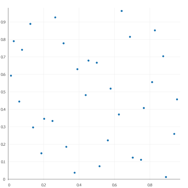
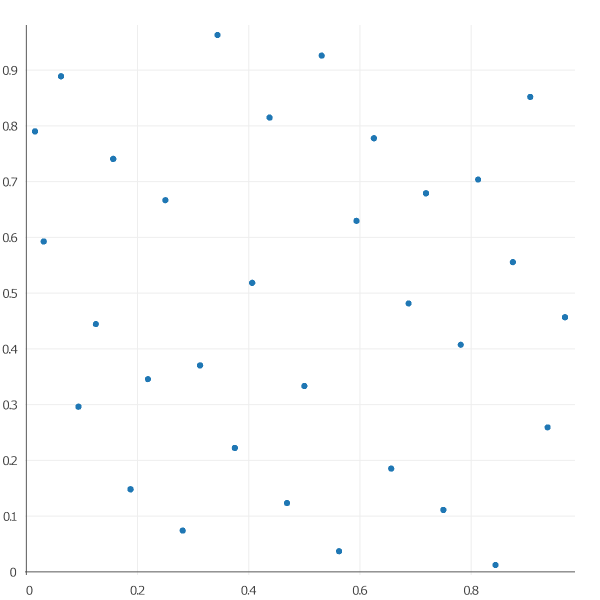
Now, let's take it for a spin. We'll leave \(b_0\) at "native" \(2\) and set \(b_1\) to \(3\) because \(1\) is invalid. Here's \(32\) points with that configuration, we'll also prune the first element of the sequence, \((0,0)\) by means of a constant offset into the sequence, because it's not very useful:

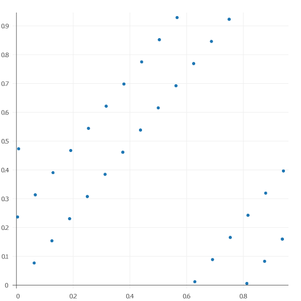
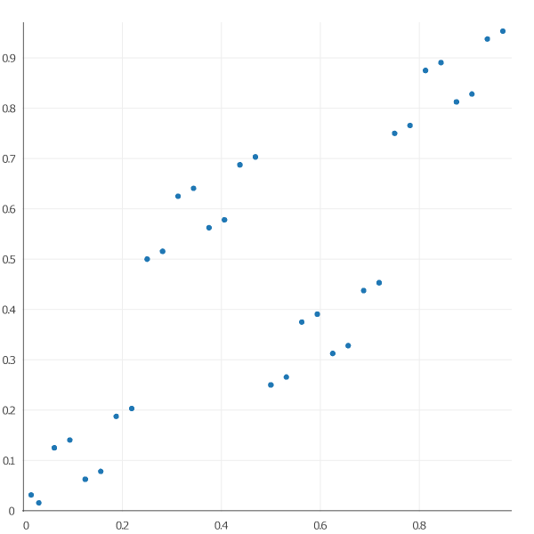
Taking the base pair \((2, 3)\) was the obvious and easiest first choice. Obviously, other choices work too with varying success. The larger the bases involved, the fewer digits are required to describe any given natural number. Let's take a look at what happens when we choose powers of \(2\) for the bases, by drawing 32 samples from a \((2, 4)\) sequence. You might guess this is a poor idea.

As you might imagine, choosing \(b_1 = 4\) is very much like using a constant offset into identical sequences, they become correlated and patterns emerge. Thus, we require the bases to be coprime, in other words, the only positive integer that divides both of them is \(1\). Anything else is equivalent to using the same base sequence with some offset. So, let's try a mutually prime pair, like \((4,3)\):

But even coprime bases will result in observable correlation once you get into the double digit bases such as \((16,13)\), as you can see below. Unlike the previous case, though, it is possible to avoid these issues but skipping a number of elements in the sequence depending on the bases used, as well as techniques involving scrambling or outright leaping.

But really, keeping the bases coprime and low is the best option for most applications. The most commonly used bases are \((2,3)\), although I suspect most people use these due to appealing to authority, rather than understanding the issues involved. This type of sequence is called the Halton sequence, after the gentleman who proposed it in 1964.

The van der Corput sequence is the lowest discrepancy sequence known to exist. It was brought forward by one Johannes Gaultherus van der Corput in 1935 and is remarkably simple in implementation as it is a transformation of the sequence of natural numbers, where each element of the latter is reflected around the radix point. The original paper is inaccessible due to old age and even when one jumps over that digital wall, there are language barriers as van der Corput was Dutch.

Equal shares

If you're not familiar with discrepancy, it's the best known measure of non-uniformity of sequences which also happens to be extremely hard to compute for any non-trivial sequence (which is to say, any useful one). To say a sequence is uniformly distributed is to say that any subinterval of the interval on which the sequence is defined receives an amount of elements that is proportional to the relative length of the interval.

One such trivial example of a uniformly distributed finite (and seemingly useless) sequence defined on the \([0,1)\) interval could be easily constructed by taking the desired number of points \(N\) and using it in the definition as \( (i/N)_{i=0}^N \) which will give us an evenly spaced point set that for \(N=10\) looks like:

Consider the subinterval \([0, 0.1)\) which is a tenth of the full interval's length (measure) on which the sequence is defined. It receives exactly a tenth of all the points (of which there are \(10\) in this case). Perfectly uniform, trivial and utterly useless... Why? First of all, it's finite due to its dependence on the number of elements in a sequence. Second of all, it's implicitly ordered in ascending order, meaning that elements come off the "queue" predictably, consider the first four elements of the sequence separately:

As expected, the upper half of the unit interval is completely devoid of elements at this point, making this a very uninteresting sequence to draw any kind of samples. Not to mention it is finite and depends on the number of points. But it is uniformly distributed, so it might be worth investigating it further. We do want our infinite sequence to be as uniformly distributed as possible. We've been looking at in the compact decimal encoding, but let's go to the "higher granularity representation" of the binary encoding (naturally, you could also choose octal or even ternary to see the same thing) and, for convenience, change \(N\) to \(8\) because a power of \(2\) in the denominator can have exact fraction representation (consider \(0.1_{(10)} \approx 0.0001100110011001101_{(2)} = 0.1000003814697265625_{(10)}\)):

Notice how the most significant bits of the fraction are the least changing ones as the sequence progresses in order. Now notice what happens when we flip those bits, making the high frequency less significant bits switch places with the low frequency higher significance bits:

Take a look how the first four elements seed the unit interval:

As you can see, much better coverage of the unit range. Again, if you look at the flipped bits, you'll notice that they're merely natural numbers in binary form reflected around the radix point, as shown in these examples: \(1_{(2)} \rightarrow 0.1_{(2)}, 10_{(2)} \rightarrow 0.01_{(2)}, 11_{(2)} \rightarrow 0.11_{(2)}, 100_{(2)} \rightarrow 0.001_{(2)}\)... This allows us to define the van der Corput sequence, without any dependence on \(N\) (thus infinite), as:

Where \(d_k(i)\) retrieves the \(k\)th digit for the reflection. Does the new sequence retain its uniform distribution? While we have no idea what is its exact discrepancy even in 2018. (or the discrepancy of any other non-trivial sequence) as it is extremely hard to compute, van der Corput and countless others have been working hard on providing a progressively decreasing upper bound on its deviance. Since its introduction in 1935., it is still the lowest discrepancy sequence in its class.

Many generalizations have been invented since in hopes of beating it, but also ones that make use of it in higher dimensions such as the Halton sequence. Given its low discrepancy results in great coverage of the domain and the associated random appearance, van der Corput sequence values are often called subrandom or quasirandom numbers and are extremely useful in many fields as a deterministic substitute for random values drawn from a uniform distribution, for example, Monte Carlo integration. I personally use the van der Corput sequence and its derivatives to solve a multitude of problems spaning anti-aliasing, terrain generation and realtime global illumination.

$$A = \frac{1}{k}\sum_{i=1}^{k}x_i$$

It is astonishing how many people use this definition, without having the slightest idea of how it works. You usually hear "Add all the elements together and divide by the number of elements - that's the average." Ask the person selling you that explanation where does the relationship stem from, you'll probably get a wall of silence, or even worse, more explanations which use the very notion they're trying to explain.

One representing the many

Let's explore this organically, which means our logic will drive us into the wall before reaching the correct answer. Suppose we have an array of a few rather random (accidentally odd) numbers:

$$R = [3, 5, 11]$$

They could be anything. Money, grades in school, irrelevant. The statement of the problem is: "How do we find out a number $n$ which relates to all inputs as close as possible?" What does it mean to lie as close as possible? It means that the absolute difference between the input and a supposed value $n$ is as low as possible. Let's formalize such a statement by trying to estimate how $n=6$ relates to all of our values:

We can see the how far $n$ is from every input. We want minimal numbers here, as small as the inputs permit (because they modulate the final output). We could spend all day searching for the smallest possible $\Delta$-difference array which is given as a function of $n$, or we could do something clever. We want the number whose distance from every input is as small as possible. Well, we could add up all the differences:

Where $k$ is the number of inputs. In the previous example, that gives us a total miss of $d(6) = 9$. We want $d(n)$ to be as small as possible which simply means to be maximally close to all of the inputs. You could track the possible solution as the lowest point which the function $d(n)$ reaches, but as the function is both linear and limited to positive values means it doesn't have a continuous derivative at the point of reflection, which is exactly the point we're looking for. Well, the only reason we used absolute values was to denote that we desire positive values, because negative distances don't make sense. What else can give us positive values, preserve order and relieve our problem of a non-continuous first derivative? Raise the equations to the power of $2$!

Well, that was quick. What have we gained? We now have our distances squared and summed, but positive. And guess what, we now have a unique peak value:

So, let's first expand our $d(n)$ before deriving and extrapolating the $n$ at $d'(n) = 0$, here are the steps:

Differentiating:

And the winner is:

Could it be? Oh, yes. That's the elusive, proper definition of an arithmetic mean. Nobody woke up one day and simply wrote out the final equation. It was an important issue to resolve, to find what is the value around which all inputs tend to be accumulating.

And that's the whole point of it, when you try to reduce the sum of accumulated squared distances by respecting all the inputs included, you will find that the value drops around the most populated areas of the number line. Also, when you have only two values, that's simply resolves down to the middle between two points on the numberline. The more inputs you have, the more precisely can you define the central tendency.