Latest posts

Efficient GPU-based occlusion culling via early-Z and indirect dispatch

Domagoj Pandza on July 4th, 2019

If a tree falls in a forest and no one is around to hear it, does it make a sound? This is a popular introductory question in philosophy, on which many have opined over the centuries. When it comes to virtual worlds, the answer is a resounding no. Out of sight, out of mind, out of processing. It will be logged, its state updated but it won't be made visible or audible for it is outside the view frustum (and audio range).

What of objects that are in the view frustum, but are completely occluded by some other, larger object? The problem of occlusion culling is a fundamental one in computer graphics and has been extensively researched, especially as it is continuously affected by advances in hardware and software.

A recap of recent history

...from the start of the century

In the early 2000s, central processors were still single-threaded and GPUs were considerably less programmable than they are today. The solution was introduced in the form of special hardware functionality to tackle occlusion culling on the GPU called "hardware occlusion queries". However, they require a ridiculously slow, error-prone, constant ping-pong match between the CPU and the GPU which considerably reduces the possible performance gain margins. The CPU has to configure the GPU for occlusion queries, submit the query data (render coarse geometry) and read back the results in order to update its indirection-heavy hierarchical structures dedicated to accelerating visibility determination and avoiding false negatives. And only then is it finally able to submit all the visible instances for rendering using the immediate mode APIs of the time (Direct3D 9.x / OpenGL 1.x+). The most successful approach of this generation of occlusion culling technology was called coherent hierarchical occlusion culling (commonly abbreviated as CHC++).

Coherent hierarchical occlusion culling in action

Sliding into the 2010s, more and more users had already acquired multithreaded microprocessors which boasted vectorization extensions as well. Tired of the cache-incoherent nature of hierarchical occlusion culling, hard-to-manage false negatives and overall latency of communicating back and forth with the GPU before even beginning to construct a frame, we turned to more CPU-centric, data-oriented methods for occlusion culling. Especially as it was already becoming more and more economical to just brute force "general" culling just by doing view frustum culling against large blocks directly on the CPUs and still run circles around methods like octree-based culling. The solution was a bit out there, we're essentially talking about software occlusion queries. They involved running a small rasterizer on the CPUs which generated a low resolution depth buffer which would then be used solely with bounding geometry to estimate occlusion by large, predefined static occluders. First commercially successful game (I am aware of) that opted for this method was DICE's Battlefield 3 running on the Frostbite engine. I have no doubt that this was directly motivated by the considerable number of Cell SPEs alongside the PPU on the Playstation 3.

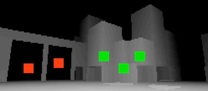
Software-rasterized low resolution depth of large, static occluders for occlusion testing.

With the arrival of true indirect dispatch allowing the GPU to compute the drawing set on its own without CPU intervention, a shift back towards hardware-accelerated occlusion culling was made. This was further bolstered by advances in temporal reprojection approaches, leading to methods where the occlusion culled set was determined using a downsampled, hierarchical depth buffer from previous frames during the advent of "next-gen" graphics APIs around 2014 and 2015.

Around that time, I had a strong itch regarding whether or not I could mix early-z testing and conservative rasterization to utilize fast hardware paths of modern GPUs to do my occlusion culling for free because there are penalties to the hierarchical approach which I deemed undesirable. Unfortunately, conservative rasterization tier support on modern GPUs was and is so bad that even Maxwell 2.0 GPUs like the GTX 980 support only tier 1 which is inadequate for the task at hand. On the other hand, my hunch about early-z subversion was right on the money. And fortunately for me, I wasn't the only one to consider it which is always helpful to avoid a considerable amount of head-scratching and writing suboptimal implementations.

Are you still there?

The main question behind all culling.

We start with the depth buffer of the previous frame. Naturally, this means the first frame will have no occlusion culling. However, unlike temporal supersampling which takes a few frames to converge, we're ready to go on the second frame. Given that efficient occlusion culling methods use oriented bounding boxes and, at best, coarse meshes to represent entities in the scene, we don't need the full resolution provided by the depth buffer which would bog down the system and eliminate the advantage.

CPU-side occlusion culling implementations utilizing software rasterization like the one behind DICE's Battlefield 3 have shown that $1/16$ resolution is more than sufficient. It is also the second most reasonable guess given that the buffer needs to be downsampled isotropically and done in one step. Downsampling is done by taking the closest (maximum when inverted) value of each 4x4 block considered, which is par for the course when it comes to analyzing depth buffers. Especially if you have done depth-sensitive ray marchers for screenspace reflections or performed something like tile-based light culling.

// Optimized for readability
#define THREAD_GROUP_DIMENSION 8

// Organize your data as you like.

struct thread_execution_information {
    uint3 thread_id : SV_DispatchThreadID;
    uint3 thread_group_id : SV_GroupThreadID;
    uint3 group_id : SV_GroupID;
    uint group_index : SV_GroupIndex;
};

[numthreads(THREAD_GROUP_DIMENSION, THREAD_GROUP_DIMENSION, 1)]
void main(thread_execution_information executing_thread_information) {

    float2 const center_offset = float2(0.5f, 0.5f);
    float2 const thread_fid = float2(executing_thread_information.thread_id.xy);
    float2 const downsampled_buffer_dimensions = 0.25f * depth_buffer_dimensions;

    // This will move us to the center of each 4x4 block within the full resolution buffer.
    float2 const downsampled_center = (thread_fid + center_offset) / downsampled_buffer_dimensions;
    if(downsampled_center.x >= 1.0f || downsampled_center.y >= 1.0f) return; // Out of bounds

    // Full resolution buffer texel size, so we can get to the centers of the surrounding
    // 2x2 blocks on which we will apply D3D12_FILTER_MAXIMUM_MIN_MAG_POINT_MIP_LINEAR,
    // to ensure there are no zero weights which would discard them from the max comparison.
    float2 const full_resolution_texel_size = 1.0f / depth_buffer_dimensions; 
    
    float block_maximums[4];
    float2 block_center_offsets[4] = { 
        float2(-1.0f, -1.0f), float2( 1.0f, -1.0f), 
        float2( 1.0f,  1.0f), float2(-1.0f,  1.0f) 
    };

    [unroll]
    for(int i = 0; i < 4; ++i) {
        float2 const center = downsampled_center + full_resolution_texel_size * block_center_offsets[i];
        block_maximums[i] = depth_buffer.SampleLevel(depth_max_sampler, center, 0).r;
    }

    // Final manual maximum determination performed, ready for reprojection.
    float downsampled_depth = max(max(max(block_maximums[0], block_maximums[1]), block_maximums[2]), block_maximums[3]);

    // ...

Downsampling the depth buffer using D3D11.2+ "MinMaxFiltering" (Tied to FL12_0 / Tiled Resources Tier 2).

Regarding Min-Max Filtering

We're relying on functionality which was originally optional with Direct3D 11.2. Specifically, the ability to do min-max sampling which is now widely supported on Direct3D 12 capable hardware. Supporting transitional hardware with primarily FL11_1 capabilities will require you to implement the downsampling the old-fashioned way.

Onto the reprojection. Just like with temporal supersampling, we only have the information which is available in screenspace. Fast camera movements will generate erroneous areas due to a myriad of reasons, stuff leaving the screen, going behind it, coming onto it, objects moving in a way that information from previous frames is invalidated etc. Good news is that occlusion culling is far less sensitive to these types of errors but that doesn't mean a free lunch, unfortunately. Since there isn't a good way to select an alternative value in those areas, the only one that can be used semi-reliably is the downsampled depth we computed in the listing above.

Credit where credit is due

The nugget in the last paragraph is due to the folks behind Deus Ex's Dawn engine. Previously, I actually used a heuristic to "content-aware out" those gaps which turned out to be unnecessarily complex. Like I said, always pays to have multiple people on the same trail, willing to share their findings.

Furthermore, as depths are non-linear and inverted (avoiding z-fighting), another concern is stuff going behind the screen because that's where depth values may "explode" and corrupt our efficiency.

    // We're in texture space right now. In Direct3D, the origin is the top-left corner.
    // In order to use the inverse projection transform, we need to go back to normalized device coordinates.
    // Depth is in the 0 to 1 range, Y axis is flipped and XY go from [-1, 1].

    float2 xy_ndc = downsampled_center * float2(2.0f, -2.0f) - 1.0f;
    float4 position_ws = mul(previous_inverted_projection_view_transform, float4(xy_ndc, downsampled_depth, 1.0f));
    position_ws /= position_ws.w; // Complete the non-linear part of the transform.

    // Using the new world position and the current projection-view transfrom, we compute 
    // the new placement position in texture space to put the reprojected depth in.
    
    // First to NDC:
    float4 reprojected_position = mul(current_projection_view_transform, position_ws);
    reprojected_position /= reprojected_position.w;
    float depth = reprojected_position.w < 0.0f ? downsampled_depth : reprojected_position.z;

    // Then to texture space:
    reprojected_position.xy *= float2(0.5f, -0.5f); 
    reprojected_position.xy += 0.5f;

    // The downsampled depth buffer has all its values initialized to 0 by default, which precludes the possibility
    // of utilizing InterlockedMin, requiring us to do some inversion gymnastics here for this to work.

    uint intermediate_depth = asuint(1.0f - saturate(depth));

    // Safest thing is to overwrite the possible hole immediately, minimizing the error (but this is a coarse approximation)
    InterlockedMax(downsampled_depth_buffer[executing_thread_information.thread_id.xy], intermediate_depth);

    // Finally store in reprojected position as well.
    int2 reprojected_position_ps = int2(saturate(reprojected_position.xy) * downsampled_buffer_dimensions);
    InterlockedMax(downsampled_depth_buffer[reprojected_position_ps], intermediate_depth);


}

Temporal reprojection followed by cleanup on aisle 3.

With the reprojected, downsampled depth buffer in tow, we're ready to subvert age old depth prepass of forward-biased approaches to occlusion culling by placing the [earlydepthstencil] attribute on the pixel shader. As you (should) know, this will force early depth testing which predicates the execution of the pixel shader. Thus, as we draw our OBBs and coarse bounding geometries, only the visible ones will actually trigger the execution of the pixel shader.

In it, we we use a simple UAV to a linear structured buffer where the "structure" are integers, fundamentally behaving like an array of booleans. It's trivial to clear this structure to $0$ by using the appropriate ID3D12GraphicsCommandList :: ClearUnorderedAccessView* Direct3D 12 API, so the final shader looks satisfyingly simple. You just use the instance IDs to index into the preallocated visibility buffer and set it to $1$. Unordered access mechanism takes care of the boatload of incoming writes.

RWStructuredBuffer<uint> visibility_buffer : register(u0);

[earlydepthstencil]
void main(uint instance_id : SV_InstanceID) {
    visibility_buffer[instance_id] = 1; // Free lunch.
}

Simplest shader you'll ever write.

All that remains is to write a custom-tailored compute shader (for your tech) which operates on every instance that passed general culling, whatever your implementation of it might be. You go through each and check them against the visibility buffer. If you determine one is visible, generate the indirect drawing information and store it in the appropriate buffer which you'll trigger from the command list later on.

However, keep in mind that errors due to temporal reprojection and even failure to rasterize small OBBs (not touching an unobstructed pixel's center) are guaranteed to introduce false negatives. Thus, you should also maintain a list of occluded instances and redraw their OBBs against the freshly built full resolution depth buffer composed of all the possible occluders after indirectly dispatching the visible instances. This entails running through a near carbon-copy of the first pass, albeit considerably simplified.

The approach works for both forward and defer biased rendering systems and integrates seamlessly. I am personally still rolling a hybrid forward-biased renderer because of my preference for delivering the option of superb spatio-temporal supersampling and elegant handling of transparency. But if your platform has considerable constraints, nobody will judge you for going deferred.

Upgrading quaternions to handle rigid transformations

Domagoj Pandza on May 30th, 2019

Mathematics

Show in single article view

In a previous article, we showed how one can arrive at quaternions. They are exceptional at handling rotations in three-dimensional Euclidean space, providing an efficient and elegant representation free of mapping singularities. However, they're not very useful when it comes to handling other affine transformations, most notably translation and scaling. Scaling can be forgiven, but translation is crucial to enabling rigid transformations and applications in many fields from robotics to computer animation.

Concerning notation

We follow the convention established previously. Lowercase letters are used to denote all quaternions $q$ except for pure quaternions $\mathbf{p}$ (no scalar component) which are marked with an upright bold letter. Unit quaternions $\hat{q}$ are marked with a hat. Given that we'll be extending quaternions in this article, further notation will be exposed as we progress.

Bootstrapping translations

We already showed that the only way to procure a "proper" rotation with quaternions (the conical transformation you're used to from linear algebra) is to compute $\mathbf{p}' = r\mathbf{p}r^*$. Thus, it is reasonable to assume that our translation transformation should assume the same format in the interest of composition with rotations. In other words, we expect $\mathbf{p}' = t\mathbf{p}t^*$. We can also assume a double translation should occur just like with rotations. However, regular quaternion multiplication is unable to perform such a feat without augmentation facilitated by changing/adding rules.

Let us focus on the $t\mathbf{p}$ part of the transform. We represent the position as a pure quaternion (zero scalar component) and assume it makes some sense to have the translation quaternion be one as well, at least for now. We need to augment quaternion multiplication in some manner to enable the translation transformation. To see what we're working with, let's lay it out:

$$ tp = \mathbf{t}\mathbf{p} =(t_xi + t_yj + t_zk)(p_xi + p_yj + p_zk) = \mathbf{t}\times\mathbf{p} - \mathbf{t}\cdot\mathbf{p}$$

Obviously, this is far from the desired outcome. One way we can try to move in the right direction is to add a real scalar component to both quaternions, of value $1$:

$$ tp = [1 + \mathbf{t}][1 + \mathbf{p}] = 1 + (\mathbf{p} + \mathbf{t}) + \mathbf{p}\mathbf{t}$$

We could live with a constant scalar part of $1$, but that last term is expectedly just pushing our original problem deeper. However, given that it is a product of our imaginary vector components, if we were to augment them with an indeterminate, say, $\omega$... We could then posit that $\omega^2 = 0$. You might see where I am going with this:

$$ \begin{split} tp &= [1 + \omega\mathbf{t}][1 + \omega\mathbf{p}] \\ &= 1 + \omega\mathbf{p} + \omega\mathbf{t} + \omega^2\mathbf{p}\mathbf{t} \\ &= 1 + \omega(\mathbf{p} + \mathbf{t}) \\ \end{split}$$

It certainly worked out, but we now need to figure out the implications of introducing the indeterminate $\omega$ into the mix. We do notice that our result is attached to it, reminiscent of the way the imaginary component of a complex number is attached to the indeterminate $i$. Our next goal, in the interest of eventually ensuring proper composition, is to complete the transform. Thus, we need to ensure $tpt^*$ doesn't fail us:

$$ \begin{split} tpt^* &= [1 + \omega\mathbf{t}][1 + \omega\mathbf{p}][1 - \omega\mathbf{t}] \\ &= [1 + \omega\mathbf{p} + \omega\mathbf{t}][1 - \omega\mathbf{t}] \\ &= 1 + \omega\mathbf{p} + \omega\mathbf{t} - \omega\mathbf{t} \\ &= 1 + \omega\mathbf{p} \\ \end{split}$$

Well, that fell apart quickly. It would appear that the conjugate here doesn't behave in the usual way. It might be prudent for us to come to terms that we're no longer dealing with regular quaternions. To test this theory, we will use a non-trivial case of rotations, but this time performed on our generalized position quaternion (to not break emerging compatibility with translation):

$$ \Large { r(1 + \omega\mathbf{p})r^* = (r + \omega r\mathbf{p})r^* = rr^* + \omega r\mathbf{p}r^* = 1 + \omega r\mathbf{p}r^*} $$

A few things of note are happening here. In the case of rotation, we desire to multiply $r$ with $p$, hence we don't attach $\omega$ to $r$ in order for them not to annihilate. Notice the part of the equation before we apply the conjugate, $(r + \omega r\mathbf{p})$. We appear to be dealing with two quaternions. One that is free and the other which is attached to $\omega$. This leads us to posit that the initially assumed scalar component in the position and translation quaternions was and is actually a quaternion itself, a real quaternion (no imaginary vector component). For lack of a better term right now, we'll call these $\Omega$-quaternions, generically specified as $Q = q + \omega q_{\omega}$. One other thing that we may hazard a guess towards from our experience so far is that any properly transformed quaternion is going to have a free component consisting of a real quaternion valued $1$ and the useful result encoded in the $\omega$-component.

Furthermore, since we're talking about two quaternions, we've been going about conjugation all wrong. It stands to reason that $Q^* = q^* + \omega q_{\omega}^*$. Applying this to our original translation transform attempt, we get:

$$ \begin{split} TPT^* &= [1 + \omega\mathbf{t}][1 + \omega\mathbf{p}][1^* + \omega\mathbf{t}^*] \\ &= [1 + \omega\mathbf{p} + \omega\mathbf{t}][1 + \omega(-\mathbf{t})] \\ &= 1 + \omega\mathbf{p} + \omega\mathbf{t} - \omega\mathbf{t} \\ &= 1 + \omega\mathbf{p} \\ \end{split}$$

It might seem like we're back to square one, but we just have to keep molding it to meet our goals. Notice that we can conjugate the $\Omega$-quaternion as before, then conjugate its constituent regular quaternions! This would result in the desired double translation by avoiding inversion while still ensuring rotation gets inverted (as it isn't affected by $\Omega$-quaternion conjugation). To differentiate $\Omega$-quaternion conjugation from regular conjugation, we use an overline. For example, the conjugate of $Q$ is then $\overline{Q}$ and the combined conjugate of $Q$ and its constituent quaternions $(q,q_{\omega})$ is thus $\overline{Q^*} = \overline{Q}^*$. While you're working out the simple proof for that on your own, you might also want to prove that $\overline{(Q_1Q_2)^*} = \overline{Q_2^*}\space\overline{Q_1^*}$. Incorporating these changes, we get:

$$ \begin{split} TP\overline{T^*} &= [1 + \omega\mathbf{t}][1 + \omega\mathbf{p}][1^* - \omega\mathbf{t}^*] \\ &= [1 + \omega\mathbf{p} + \omega\mathbf{t}][1 - \omega(-\mathbf{t})] \\ &= 1 + \omega(\mathbf{p} + 2\mathbf{t}) \end{split}$$

We're almost ready to combine a rotation and a translation into a rigid transformation, and compute its conjugate. However, to verify the properties of rigid transformations, we will have to generalize the notion of the quaternion norm, usually computed a as $||q|| = \sqrt{qq^*}$. So, we compute:

$$ \begin{split} (q_0 + \omega q_{\omega})(q_0 + \omega q_{\omega})^* &= (q_0 + \omega q_{\omega})(q_0^* + \omega q_{\omega}^*) \\ &= q_0q_0^* - \omega q_0 q_{\omega}^* + \omega q_{\omega} q_0^* \\ &= ||q_0||^2 + \omega(q_{\omega} q_0^* + q_0 q_{\omega}^*) \\ &= ||q_0||^2 + \omega2\langle q_0, q_{\omega}\rangle \\ \end{split}$$

At this point, we need to take a squared root while being considerate of $\omega$. To this end, we rephrase the problem generically: $(a + \omega b)^2 = a^2 + \omega 2ab = c + \omega d$. From this, it follows trivially that $a = \sqrt{c}$ and $b = d / \sqrt{4c}$. Notice that when the constituent quaternions are real, this looks a lot like something that is kin to complex numbers. We'll cover this in the next section. Armed with these new relations, we conclude:

$$ ||Q|| = \sqrt{QQ^*} = ||q|| + \omega\frac{\langle q, q_{\omega}\rangle}{||q||} $$

We now know that the only way to have a unit $\Omega$-quaternion is for the inner product of its constituent quaternions to resolve to $0$. Vanilla rotation is encoded with unit quaternions and has a zero quaternion in the omega component when extended to $\Omega$-quaternions as it performs rotation directly through vanilla multiplication. Thus, the inner product is $0$ and it remains unit here as well. On the other hand, $\Omega$-quaternions encoding translation are composed of a real and pure quaternion which results in their inner product being $0$ as well, making the $\Omega$-quaternion unit if and only if the real quaternion is valued $1$. A fundamental property of normed division algebras is $||qp|| = ||q||||p||$ and this extends to $\Omega$-quaternion, allowing us to surmise the composition of rotation and translation will be a unit $\Omega$-quaternion. We now compute the composition $TR$:

$$\Large{TR = [1 + \omega\mathbf{t}][\hat{r} + \omega 0] = \hat{r} + \omega\mathbf{t}\hat{r}}$$

Its conjugate $(TR)^* = R^*T^*$ is given by $\hat{r}^* - \omega\hat{r}^*\mathbf{t}$ which allows us to compute the norm and confirm that it is indeed unit:

$$\Large{ \begin{split} ||TR||^2 &= [\hat{r} + \omega\mathbf{t}\hat{r}][\hat{r}^* - \omega\hat{r}^*\mathbf{t}] \\ &= \hat{r}\hat{r}^* - \omega\hat{r}\hat{r}^*\mathbf{t} + \omega\mathbf{t}\hat{r}\hat{r}^* \\ &= 1 - \omega\mathbf{t} + \omega\mathbf{t} = 1 \\ \end{split}}$$

Finally, we work out a rigid transformation $(TR)P\overline{(TR)^*}$ of a point $P$ and show mathematically that the point is indeed double rotated then double translated into its transformed position:

$$\Large{\begin{split} (TR)P\overline{(TR)^*} &= [\hat{r} + \omega\mathbf{t}\hat{r}][1 + \omega\mathbf{p}][\hat{r}^* + \omega\hat{r}^*\mathbf{t}] \\ &= [\hat{r} + \omega\hat{r}\mathbf{p} + \omega\mathbf{t}\hat{r}][\hat{r}^* + \omega\hat{r}^*\mathbf{t}] \\ &= [\hat{r} + \omega(\hat{r}\mathbf{p} + \mathbf{t}\hat{r})][\hat{r}^* + \omega\hat{r}^*\mathbf{t}] \\ &= \hat{r}\hat{r}^* + \omega\hat{r}\hat{r}^*\mathbf{t} + \omega(\hat{r}\mathbf{p}\hat{r}^* + \mathbf{t}\hat{r}\hat{r}^*) \\ &= 1 + \omega\mathbf{t} + \omega(\hat{r}\mathbf{p}\hat{r}^* + \mathbf{t}) \\ &= 1 + \omega(\hat{r}\mathbf{p}\hat{r}^* + 2\mathbf{t}) \\ \end{split}}$$

And there you have it! A rotation followed by a translation, stored in the omega component of our $\Omega$-quaternion. Historically, this result was first recorded in a journal by one Wiliam Kingdon Clifford in 1873. He based his work on Hamilton's quaternions, meaning he also adopted a lot of his preconceptions, including the iffy notion of dividing vectors which was discarded in modern mathematics, but is pervasive in the paper. He originally named the indeterminate $\omega$ which we've used in our derivation here as a nod to him. In his self-proclaimed "preliminary sketch", Clifford named his precursor "biquaternions". This work would later be picked up by Eduard Study who moved them in the direction of what would eventually become known as a dual quaternions. Our $\Omega$-quaternions are dual quaternions. Like us, Study was interested in applying this construct for rigid transformations. In modern times $\epsilon$ has superseded $\omega$ as the indeterminate element. In the next article, we will extract the notion of dual numbers from our "organically derived" dual quaternions... Which will allow us to consider some interesting properties dual numbers have over their "singular" counterparts.

Heuristic for energy compensation in single-scattering microfacet BSDFs

Domagoj Pandza on August 28th, 2018

Computer Graphics

Show in single article view

You're reading the series on handling multiple scatter events on a statistical microsurface

In this article, we dismantle the existing single-scattering microfacet BSDF model to find a quick and dirty heuristic which is good enough for practical, realtime applications. This means the primary focus here is energy compensation rather than simulating multiple scattering, even though we do manage to get a decent approximation of it.

This is one of those articles I've been wanting to write for a while now. My initial approach to correcting the issue, predecessor of the one described in the following text, was deemed too brazen in its approximation. I've had quite a while to rethink it. I still don't feel it's properly solved. What's the problem? Microfacet BSDFs have been losing energy for decades! Sweet clickbait, but it's true. Up to 60% of it at extreme microsurface roughness which has a serious impact on visual quality. If you're in the computer graphics research circles, this is not news to you.

Since 1976 (even 1967), we've knowingly assumed that only a single bounce on the statistical microsurface occurs. Every subsequent one is modeled as "lost to the void". The focus back then was making sure we don't create energy. For this purpose, a very reliable model for microsurface shadowing and masking was introduced by Smith in 1976. All of this led to us collectively creating and abetting a light trap. The price was mostly paid on dieletrics and conductors at high surface roughness levels, as they grew dimmer and duller. The following equation outlines the problem unequivocally:

$$\int_{\Omega^+} \frac{D(h)G(\omega_i, \omega_o, h)}{4 \langle w_i, n \rangle \langle w_o, n \rangle } \langle w_i, n \rangle d\omega_i \neq 1$$

In this series of articles, I'll share how I approached rectifying it since the beginning of this decade, as well as ease you into how I changed my approach over the years following research performed by Heitz, Turquin and others. Don't worry, we'll cover derivations and computations of all the concepts introduced. If you're not familiar with microfacet BRDFs, Torrance-Sparrow paper from 1967 is one of the rare papers which actually includes a decent mathematical derivation. Only prerequisite is that you're familiar with spherical trigonometry.

Energy loss as a function of increasing roughness $r$.

Approaching the problem...

...via savage mathematical manipulation

We omit the Fresnel factor to ensure perfect reflectance at any angle in order to observe and fix the problem. Assuming a constantly lit environment, this allows us to verify that, indeed, light falling onto the hemisphere above the evaluated point is not being completely reflected back into the environment by a single-scattering microfacet BRDF as roughness rises. My first idea was adhoc scaling as a function of roughness, however, I disliked the result.

From there, I tried changing my approach to restating the BRDF to account for the lost energy by just shooting the difference back out in every direction scaled by the distribution. Naturally, this isn't easy to justify physically as it is a mathematical transformation, we're not actually wading through a statistical microsurface. Heitz did in 2016, but we'll get to that later. The integral from the introduction can be restated as a function of how much reflectance is dished out in the direction $\omega$:

$$ E(\omega) = \int_{\Omega^+} \rho(\omega, \omega_i) \langle w_i, n \rangle d\omega_i$$

This allows us to specify the constraints necessary for our modified "multi-scattering" BSDF:

$$ E_{\mathbf{first}}^{F=1}(\omega) + E_{\mathbf{multi}}^{F=1}(\omega) = 1$$

Simple enough, let's work through it. From this point forward, the superscript will no longer appear because it's cumbersome.

On expecting unity

If you're confused why we're expecting $1$ here, you need to focus on the fact that we're doing our measurements in a constantly lit environment with a "material" where both single- and multi-scattering Fresnel is currently $1$. As there are no gaps in the environment, the entire lobe is perfectly saturated.

We expect it to scatter 100% of the incoming light through the solid angle centered on $\omega$, the direction of the camera/eye/sensor. From every direction within the lobe, it'll take a variable percentage of the incoming "light" which should, over the entire lobe, reach unity.

$$ \int_{\Omega^+} \left( \frac{D(h)G(\omega_i, \omega, h)}{4 \langle w_i, n \rangle \langle w, n \rangle } + \rho(\omega, \omega_i) \right) \langle w_i, n \rangle d\omega_i = 1$$

This "trick" enables us to see the percentage of light falling onto the specular lobe that gets scattered in the $\omega$ direction and the losses incurred by ignoring multiple scattering events. It is often referred to it as the albedo (here Fresnel is $1$). Thus, we need to figure out what $\rho$ should be.

Shuffle it around a bit, into a form where we'll be able to scam the integral into doing what we want. Just to emphasize for those who get bamboozled by the following sausage is that it is just $E_{\mathbf{multi}}(\omega) = 1 - E_{\mathbf{first}}(\omega)$ laid bare:

$$ \int_{\Omega^+} \rho(\omega, \omega_i) \langle w_i, n \rangle d\omega_i = 1 - \int_{\Omega^+} \frac{D(h)G(\omega_i, \omega, h)}{4 \langle w_i, n \rangle \langle w, n \rangle } \langle w_i, n \rangle d\omega_i$$

We need to fit a function $\rho$ which will resolve the left side to what we see on the right side, as such, it can be expressed as a product of a currently unknown number $N$ of factors, each potentially a function of $\omega$ and $\omega_i$:

$$\Large \rho(\omega, \omega_i) = \prod_{i=0}^{N} X_{i}(\omega, \omega_i) $$

It is not hard to guess what our first factor will be, pretty much the right side which will allow us to focus on forcing the integral to dissolve:

$$ \left[1 - E_{\mathbf{first}}(\omega)\right]_{\rho} \int_{\Omega^+} \left[\prod_{i=1}^{N} X_{i}(\omega, \omega_i)\right]_{\rho} \langle w_i, n \rangle d\omega_i = 1 - E_{\mathbf{first}}(\omega)$$

To get a grasp of what's going on, we're going to change our variables to deal with the unit hemisphere in a way which is directly computable. Furthermore, we also dole out the normalization factors necessary after we process the outer integral:

$$2\pi \left[ \frac{1 - E_{\mathbf{first}}(\theta)}{2\pi} \right]_{\rho} \int_{0}^{\pi/2} \left[ \prod_{i=3}^{N} X_{i}(\theta, \theta_i)\right]_{\rho} \cos(\theta_i) \sin(\theta_i) d\theta_i = 1 - E_{\mathbf{first}}(\theta)$$

Solid angles and surfaces

The infinitesimal patch of area on the unit hemisphere which subtends the solid angle centered around a direction $\omega$ can be visually derived to be $\sin(\theta) d\theta d\phi$. Range is trivially limited to a full sweep of the surface of the hemisphere. As we have no azimuthal dependence here, we can process the outer integral immediately.

Now, you might be tempted to guess the remainder of the product defining $\rho$ right away, to be something along the lines of:

$$ \rho(\theta, \theta_i) = \frac{1 - E_{\mathbf{first}}(\theta)}{\pi^2\sin(\theta_i)\cos(\theta_i)} $$

Cheeky, but no. You may be scratching your head as to why. You've just added a portion of the parametrization of the integral into the denominator of our multi-scattering function and its respective normalization. Change the variables from $d\theta_i$ to $du_i$ where $u_i(\theta_i) = \cos\theta_i$ and watch the house of cards crumble. Awkwardly floating sine alongside now irrelevant normalization factors. How about something like this instead:

$$\rho(\theta, \theta_i) = \frac{1 - E_{\mathbf{first}}(\theta)}{2\pi\int_{0}^{\pi/2} E(\theta_i) \cos(\theta_i) \sin(\theta_i) d\theta_i} E(\theta_i)$$

$$\frac{1 - E_{\mathbf{first}}(\theta)}{\int_{0}^{\pi/2} E(\theta_i) \cos(\theta_i) \sin(\theta_i) d\theta_i} \int_{0}^{\pi/2} E(\theta_i) \cos(\theta_i) \sin(\theta_i) d\theta_i = 1 - E_{\mathbf{first}}(\theta)$$

This was something I could precompute and put in the denominator as a normalization factor alongside $2\pi$, in my initial approach. While my intention was not to give any particular semantics to this particular integral, it looked like a weighted average of the albedo where the weights were a function of the cosine of the angle (essentially direction where light is shot out)... It's just missing the weight scaling factor:

$$\frac{\int_{0}^{\pi/2} E(\theta_i) \cos(\theta_i) \sin(\theta_i) d\theta_i}{\int_{0}^{\pi/2} \cos(\theta_i) \sin(\theta_i) d\theta_i} = \frac{\int_{0}^{\pi/2} E(\theta_i) \cos(\theta_i) \sin(\theta_i) d\theta_i}{-\int_{1}^{0} u du} = 2\int_{0}^{\pi/2} E(\theta_i) \cos(\theta_i) \sin(\theta_i) d\theta_i$$

And we can pretend the $2$ out of our normalization is the weight scaling factor, just call it $\bar{E}$:

$$\Large\rho(\theta, \theta_i) = \frac{1 - E_{\mathbf{first}}(\theta)}{\pi\bar{E}} E_{\mathbf{first}}(\theta_i)$$

What of the Fresnel factor in this approximate multiscattering framework?

Here's the deal, precise multiple "anything" is complex to do online, especially when a statistical microsurface is involved, as we're essentially talking about running a stochastic process for an accurate result. We simply cannot afford it. It's conceptually trivial, but implementation is nigh impossible. So, we give up? No, we just need "the gist" of the effect, visual plausability.

Thus, let's assume its behavior is diffuse (as in ideal Lambertian diffuse, view direction independent). An extreme approximation, but it's something. You take a Fresnel function and take its cosine-weighted average over the unit hemisphere, giving you a mean representative of the whole which can be used in this diffuse paradise of ours. Haha, I know, a stretch. But it really doesn't matter much, single-scattering Fresnel term is the most important one here.

$$\bar{F} = 2\int_{0}^{\pi/2} F(\theta_i) \cos(\theta_i) \sin(\theta_i) d\theta_i$$

Since we're not actually tracing through the microsurface, what percentage of reflected light do we assume escapes the microsurface? Conveniently, we previously ran into a possible value here, $\bar{E}$. It's the representative mean of the fraction of light (albedo) being shot in the view direction. So, it's the light that escapes the surface, right? So, let's say that's the percentage of light that escapes on every bounce, modulated by the average Fresnel factor. So, the first bounce would send out $(1- \bar{E})\bar{F}$ in every other direction (and we assume it hits the microsurface again). That means that the remaining $1 - \bar{E}$ percentage of light is coming in "tinted" for the second hit.

Every second bounce can then be modeled singularly as sending out an $\bar{E}\bar{F}$ percentage of light in the view direction... Of the incoming $(1 - \bar{E})\bar{F}$ percentage, $\bar{E}\bar{F}(1 - \bar{E})\bar{F}$ (remember, diffusely reflected from the first hit). Extend this to the $n$-th bounce $\bar{E}\bar{F}\left(1 - \bar{E}\right)^n\bar{F}^n$ and you've got yourself a trivial geometric series which neatly converges. Only correction? Yes, the first bounce has to go as it is accounted for in the single-scattering "regular" BSDF:

$$F_{\mathbf{multi}} = \bar{E}\bar{F} \sum_{i=1}^{\infty} \left(1 - \bar{E}\right)^i\bar{F}^i $$

$$F_{\mathbf{multi}} - \left(1 - \bar{E}\right)\bar{F} F_{\mathbf{multi}} = \bar{E}\bar{F}^2 \left(1 - \bar{E}\right) $$

$$F_{\mathbf{multi}} = \frac{\bar{E}\bar{F}^2 \left(1 - \bar{E}\right)}{1 - \left(1 - \bar{E}\right)\bar{F}}$$

While this is now not repeating the single-scattering Fresnel, it is messing up the multiscattering albedo when perfect reflectance is assumed ($\bar{F} = 1$) as it resolves to $1 - \bar{E}$ which means you need to scale it down by the same amount to get back to $1$ (expected behavior). And this concludes this particular approximation of multi-scattering Fresnel incorporation.

Putting it all together

...And drawing a few conclusions

With all of this in mind, we can now augment any microfacet BSDF with an energy compensation term which is essentially approximating multiple scattering:

$$f_{\mathbf{brdf}}(\omega, \omega_i) = \frac{ D(h)G(\omega_i, \omega, h)F(\omega_i, h)}{4 \langle w_i, n \rangle \langle w, n \rangle } + \frac{\bar{F}^2}{\pi} \frac{1 - E_{\mathbf{first}}(\omega)}{ 1 - (1 - \bar{E})\bar{F}} E_{\mathbf{first}}(\omega_i)$$

In the next article, we'll be covering how the integrals are precomputed and/or fitted into the budget of a realtime application (pun intended), especially incorporating Fresnel into the mix in a way where the look-up tables won't be "unnecessarily multidimensional" and prohibitively expensive. As it stands now, it's non-trivial to compute, to say the least. To give you a taste of what we'll be doing, here's the albedo function of the single-scattering microfacet BSDF (with $F=1$) encoded as a two dimensional image (horizontally a function of angle, vertically a function of roughness):

$E_{\mathbf{first}}(\omega)$ precomputed into a 2D texture. You could even get away with a LUT as small as 16x16 given how smooth it is.

We'll have to roll up our sleeves to get Fresnel into the equation (pun intended) in a way that isn't at odds with practicality that a realtime system needs. Once we finalize that, we will jump into the work of Turquin who had a pretty interesting hot take on an approach of this flavor (of which Sony's Imageworks people are also proponents of)... He, interestingly, opted in to variably scale the single-scattering BSDF instead of manually developing a secondary term like we just did. And if you'd like to see a "before/after" image, I've got you covered:

The difference is rather striking at high roughness!

The furnace differential at high roughness is the best argument for approximating multiscattering.