Latest posts

Deriving Bézier curves and de Casteljau's algorithm from "scratch"

Domagoj Pandza on July 27th, 2020

Motivation and the usual notes

While I was discussing the finer points of my GPU-based vector graphics system, a few friends expressed annoyance with the lack of didactic exposition regarding crucial concepts behind vector graphics, among other things. The primary argument is that most literature assumes, through ignorance, laziness or comfortable complancy, that the mathematics behind Bézier curves are sufficient to present in their final form. Let's fix that.

Passed initial nerd review and is now available to the general public. I'll do some diagrams when I feel like it.

If you asked your typical programmer about Bézier curves, you'd likely find it difficult to differentiate their answer from the general "wisdom" available online, usually on websites with non-existent CSS. In other words, a truckload of circular and poorly motivated reasoning which assumes foreknowledge of the subject to derive it, positing results ahead of the premise. As such, there is little intuition and satisfaction to be gained from any such website, book or programmer. The story of Bézier curves is a fascinating one, and a lot messier than most sources make it out to be. The way they were originally derived is obscured in the publications as a result of the process best illustrated by this hilarious meme masquerading as a paper.

The problem with modern exposition of the subject is that the original spirit of the derivation was obfuscated in favor of an impressive showcase in terms of relations that were uncovered towards the end. As most programmers don't invest much thought in the why and how beyond gaining the ability to use it, nuance is easily lost. As such, "de Casteljau's algorithm" is taken as gospel and statements like "Bézier curves are based on Bernstein polynomials" are common place. They are related to them and are mathematically equivalent, meaning that properties studied on the latter can be used to inform the former. That does not mean they're derived from them or provide any kind of intuition or basis on how to reason about Bézier curves. Their properties are used to prove and generalize what our intuition is implying in simpler cases. To put it differently, there is no clear path to Bernstein polynomials without prior knowledge of the relationship between the two. Otherwise you could say that Bézier curves are based on the binomial distribution and probability theory.

Luckily for you, I am one particularly ridiculous nerd who likes to independently arrive at the constructs he uses in his daily work. So, let us table Bernstein polynomials for now and we'll get back to them organically, once the link arises naturally.

A brief history with some spicy drama

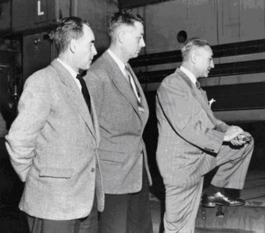
Bézier is the feller in the middle.

It was indeed Pierre Bézier who first popularized the application of these curves in computer aided design of automotive bodies while working at Renault in the 1960s. Renault at the time didn't have a gag order on research disclosure, which allowed Bézier to get his name attached to them under the "I was first to say I was first here" doctrine.

The primary historical reference is still the one by Bézier from a conference at the University of Utah in 1972, a university now famous in the computer graphics community for many contributions to the field and the home of the Newell teapot.

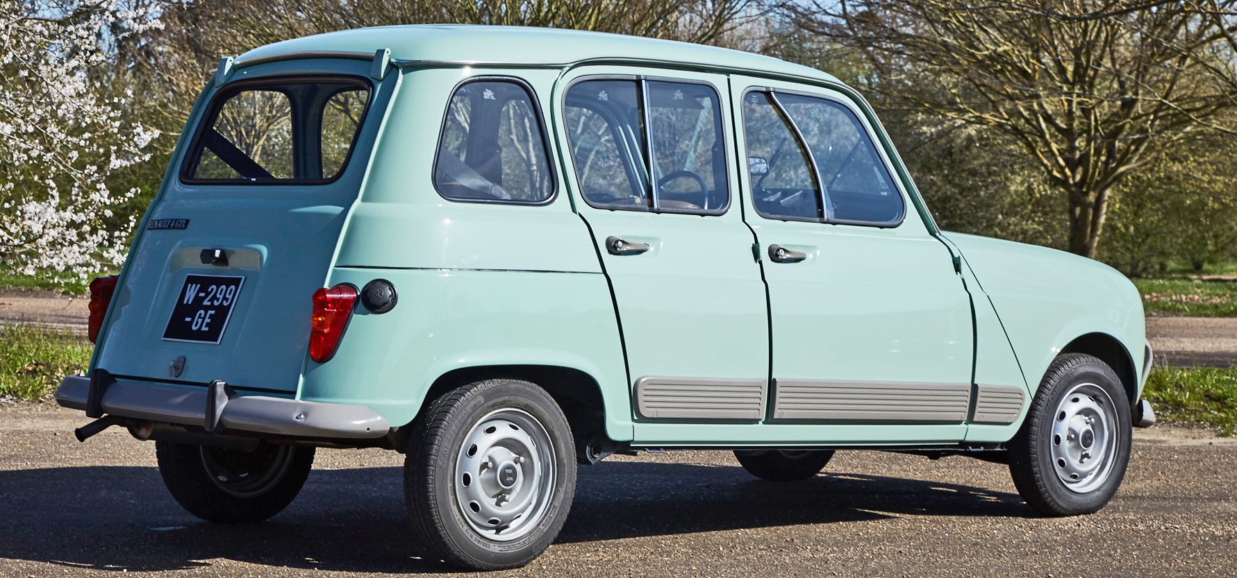
Brought to you by curvy curves.

The thing is... There was another gentleman going by the name of Paul de Casteljau who also worked at a French automotive giant, Citroën... Who claimed to have developed the same curves for the same purpose in the late 1950s, but was barred from publishing his research. Ouch. Now, I am not saying de Casteljau didn't like Bézier much, but he didn't like him. Probably because Bézier patented his life's work. Much like the feud between Newton and Leibniz, a lot of sparks flew here. By the time this was public knowledge, the industry had pretty much associated Bézier with the curves...

The consolation prize attributed to de Casteljau was the "algorithm" used for evaluating the curves. The "algorithm" is merely an unavoidable fact of life, a trivial transformation of the curve equation, and Bézier had to have derived it himself to derive an actionable mathematical basis. While it stings, it's just yet another example of Stigler's law of eponymy, itself a necessity due to the proven possibility of multiple discovery.

Connecting the dots

...one control point at a time.

To achieve anything of note in life, one needs a motivation. One look at curves in analytic geometry and you can see just how much a hassle it is to control/shape the curves intuitively, making our motivation rather clear; finding a way to intuitively control curves as a function of their endpoints and the associated tangent vectors which can be transformed into control points of some sort.

Linear Bézier curve

Our starting point is fundamental analytic geometry and the first construct introduced in analytic geometry is the line. It is fairly trivial to recover a line that goes through two points:

$$\begin{split} y &= \frac{ \mathbf{P}_{1y} - \mathbf{P}_{0y } }{\mathbf{P}_{1x} - \mathbf{P}_{0x}} (x - \mathbf{P}_{0x}) + \mathbf{P}_{0y} \\ &= \frac{ \mathbf{T}_{y} }{\mathbf{T}_{x} } (x - \mathbf{P}_{0x}) + \mathbf{P}_{0y} \\ \end{split}$$

It can be quickly rearranged into a parametric equation as a function of $t$ limited on a $[0,1]$ range:

$$\Large{\begin{split} \mathbf{P}(t) &= \mathbf{P_0} + t(\mathbf{P_1} - \mathbf{P_0}) \\ &= (1-t)\mathbf{P_0} + t\mathbf{P_1} \\ \end{split}}$$

In the context of Bézier curves, this is the linear Bézier curve. Stating the obvious, but it is also the expression for linear interpolation.

The limit of "first principles"

I thought about outlining, in excruciating detail, how one arrives at this parametric line equation. However, if the reader is unable to recover the linear interpolation equation on their own, reading this article may be a premature activity.

Quadratic Bézier curve

Don't get spoiled by the triviality exhibited so far as we're going up a degree. The first proper curve one is introduced to is usually the ubiquitous parabola. Specified in slope-intercept form, it's $y = a_2t^2 + a_1t + a_0$. If you transform it a bit, you get $y = (a_2t + a_1)t + a_0 = a(t)t + a_0$. The parabola is, thus, what happens when you linearly vary the highest degree coefficient of a line (the directional one). Thus, the derivative of a parabola is a line. As a parabola exhibits mirror-symmetry, the derivative at two points on opposite sides will be mirrored (going up, going down). In other words, they are correlated and it is possible to express the tangents as a function of the end points and a third, shared control point.

While we expressed a linear Bézier curve rather intuitively and satisfyingly by linearly interpolating its end points, the quadratic Bézier curve will not yield as easily. It does have a satisfying analogue; we can elegantly express its derivative at any point as a linear interpolation between the two endpoint "velocity vectors" or tangents specified, due to reasons elaborated in the previous paragraph, as $\mathbf{T_0} = \mathbf{P_1} - \mathbf{P_0}$ and $\mathbf{T_1} = \mathbf{P_2} - \mathbf{P_1}$:

$$\Large{\begin{split} \mathbf{P}'(t)/2 &= \mathbf{T_0} + t(\mathbf{T_1} - \mathbf{T_0}) \\ &= (1-t)\mathbf{T_0} + t\mathbf{T_1} \\ \end{split}}$$

If you're not sure why there is a factor of $1/2$ in there, it follows from the fact that the derivative of $x^2$ is $2x$. You have to be mindful of the established rules while we're playing this constructive game. By integrating this and solving for the $c$ (you're right, it's $\mathbf{P}_0$), we recover $\mathbf{P}(t)$:

$$\Large{\begin{split} \mathbf{P}(t) &= 2\int \mathbf{T_0} + t(\mathbf{T_1} - \mathbf{T_0}) \space dt \\ &= 2t\mathbf{T_0} + t^2(\mathbf{T_1} - \mathbf{T_0}) + c \\ &= 2t\mathbf{T_0} + t^2(\mathbf{T_1} - \mathbf{T_0}) + \mathbf{P}_0 \\ \end{split}}$$

And just like that, we have the quadratic Bézier curve. If you swap in the control points, you have a very easy way of evaluating quadratic curves which is sufficient for specifying glyphs of fonts for text rendering. However, to go beyond, one can perform mental gymnastics like the ones we did here. Or we can look for some pattern here. As we have derived the linear Bézier curve as a simple linear interpolation of the end points and the quadratic Bézier curve by noticing its derivative can be expressed in terms of a linear interpolation of the velocity vectors... It just might lead to some generalization if we unroll everything and try to rearrange a bit:

$$\begin{split} \mathbf{P}(t) &= \mathbf{P}_0 + 2t(\mathbf{P_1} - \mathbf{P_0}) + t^2(\mathbf{T_1} - \mathbf{T_0})\\ &= \mathbf{P}_0 + t\mathbf{T_0} + t(\mathbf{P_1} - \mathbf{P_0}) + t^2(\mathbf{T_1} - \mathbf{T_0}) \\ &= \mathbf{P}_0 + t\mathbf{T_0} + t\left[ \mathbf{P_1} - \mathbf{P_0} + t(\mathbf{T_1} - \mathbf{T_0}) \right] \\ &= \mathbf{P}_0 + t\mathbf{T_0} + t\left[ \mathbf{P_1} + t\mathbf{T_1} - (\mathbf{P_0} + t\mathbf{T_0}) \right] \\ \end{split}$$

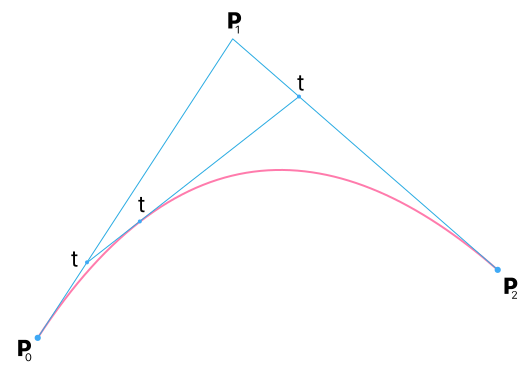
Well, it's a triple linear interpolation, isn't it? The result is the linear interpolation of the linear interpolation between the first end point and the control point and the linear interpolation of the control point and second end point. Given that is true, it can be trivially rephrased as:

$$\begin{split} \mathbf{P}(t) &= (1-t) \left[ (1-t)\mathbf{P_0} + t\mathbf{P_1}\right] + t\left[(1-t)\mathbf{P_0} + t\mathbf{T_0} \right] \\ &= (1-t)^2\mathbf{P_0} + 2(1-t)t\mathbf{P_1} + t^2\mathbf{P_2} \end{split}$$

That is beginning to look an awful lot like the algorithm attributed to de Casteljau. And this is one way of arriving at it that I find particularly intuitive. Rearrangement following the result of an intuitive base assumption. You don't go trying "well, maybe we do triple interpolation" without any real argument to do so. Especially because you need to understand how $t$ plays into it. I mean, you can, but stumbling onto it is not a good look. At least, as far as I'm concerned.

Cubic Bézier curve

If a linear Bézier curve can be represented with a single linear interpolation, a quadratic with three... Well, now we have a leg to stand on and posit that a cubic could be represented with six, using the same tree-like approach! It also stands to reason there will be two control points aiding the two end points:

$$\Large{\begin{split} \mathbf{P}_{0 \rightarrow 1}(t) &= (1-t)\mathbf{P_0} + t\mathbf{P_1} \\ \mathbf{P}_{1 \rightarrow 2}(t) &= (1-t)\mathbf{P_1} + t\mathbf{P_2} \\ \mathbf{P}_{2 \rightarrow 3}(t) &= (1-t)\mathbf{P_2} + t\mathbf{P_3} \\ \end{split}}$$

$$\Large{\begin{split} \mathbf{P}(t) &= (1-t) \left[ (1-t)\mathbf{P}_{0 \rightarrow 1}(t) + t\mathbf{P}_{1 \rightarrow 2}(t)\right] \\ &+ t\left[(1-t)\mathbf{P}_{1 \rightarrow 2}(t) + t\mathbf{P}_{2 \rightarrow 3}(t) \right] \\ \end{split}}$$

Which can be further rearranged and expressed in terms of the points as:

$$\Large{\begin{split} \mathbf{P}(t) = (1-t)^3\mathbf{P_0} &+ 3(1-t)^2t\mathbf{P_1} \\ &+ 3(1-t)t^2\mathbf{P_2} + t^3\mathbf{P_3} \\ \end{split}}$$

Those are some mad binomial expansion vibes. Or, if you have a stronger background in mathematics to contrast against, Bernstein polynomials come to mind. But notice how we didn't need Bernstein polynomials to define the curves underlying all of modern vector graphics. For completeness and generalization, we are going to go there, though.

Deriving Bernstein polynomials to take us the rest of the way

Now is the time to bring up the relationship with Bernstein polynomials. The reason we turn to Bernstein is because his work simplifies our path to generalization. This is motivated by the observation that we can transform our parametric curve equations into the Bernstein form. Don't worry, I'll ease you into it.

Where to begin? Alright, at the end of the 19th century, one very useful mathematical curiousity was whether or not we could approximate any reasonably smooth function with a polynomial to arbitrary precision, whether it is possible to find a polynomial $p(x)$ for which it holds $|f(x) - p(x)| < \epsilon$ for any $x$ on the $[0,1]$ range. The range is sufficient as any function of interest delimited on $[a, b]$ can be translated and scaled to it. The first person to publicly prove this was Weierstrass when he was 70 years old (!), hence why the theorem bears his name.

Sergei Bernstein was a Russian mathematician who lived in a time when today's Stone-Weierstrass theorem was just the Weierstrass theorem and one of his many contributions to mathematics was a probabilistic proof of said theorem in 1912 based on Bernoulli trials, contrasting the constructive one originally proposed by Weierstrass himself. Bernstein argued, in a short one-page paper written in French, that you can subvert the calculation of the expected value of a binomial distribution and the weak law of large numbers in order to prove the Weierstrass theorem.

I have already covered deriving the binomial distribution years ago, which means that you have sufficient information on this website to understand the proof I'm about to outline.

From my other article, or from your past studies, we know that the expected value $\mu$ of the binomial distribution is

$$ \mu = \sum_{k=0}^{n} { k \space {n \choose k} x^k(1-x)^{n-k} } = nx$$

As it is a discrete distribution, another little, however obvious, tidbit is important to explicitly note:

$$ \sum_{k=0}^{n} { \space {n \choose k} x^k(1-x)^{n-k} } = 1$$

Why is this relevant here? Because we can then setup $p(x)$ as

$$ p(x) = E_n = \sum_{k=0}^{n} { f\left(\frac{k}{n}\right) {n \choose k} x^k(1-x)^{n-k} }$$

and the following will be valid

$$\large{ f(x) - p(x) = \sum_{k=0}^{n} { \left[f(x) - f\left(\frac{k}{n}\right)\right] {n \choose k} x^k(1-x)^{n-k} }}$$

When $k/n$ is close to $x$, the $E_n$ above clearly approximates $f(x)$. What about everywhere else? A well-behaved function has a global maximum $M$ on any delimited range, the worst case scenario is that our $p(x)$ will miss by a maximum of $2M$. Why twice the global maximum? Imagine being at the sea floor (below sea level, yes?) looking up at a mountain. $2M$. At worst, $M$ to clear the sea and $M$ to reach the top of the mountain.

How do we quantify these conditions? We split the problem on $x$. Continuity of the function guarantees that we can define the values $\epsilon$ and $\delta$ as

$$ |x - x'| \leq \delta \implies |f(x) - f(x')| < \epsilon/2 $$

We can restate it in terms of the maximum $f_{M}(x)$ and the minimum $f_{m}(x)$, defined on the interval $(x - \delta, x + \delta)$. It trivially follows that $f_{M}(x) - f(x) < \epsilon/2$ and $f(x) - f_{M}(x) < \epsilon/2$. Armed with these relations, we can start playing with constraining the expected value (which is $p(x)$ aliased as $E_n$). There's two outcomes, $|x - k/n| < \delta$ and $|x - k/n| \geq \delta$. The expected value is, therefore, constrained by the weighted average of the two on both ends, weight being the probability $q$ that $|x - k/n| \geq \delta$:

$$ (1-q)f_{m}(x) - qM < p(x) < (1-q)f_{M}(x) + qM$$

Now, that $n$ in the denominator comes handy. We can push $n$ so high that $q$ dwindles to a point where it'll be smaller than our carefully chosen constraint of $\epsilon/(4M)$. If you expand the previous equation's minimum and maximum expressions in terms of $f(x)$ and replace $q$ with our constraint, everything collapses to

$$ f(x) - \frac{\epsilon}{2} - \frac{2M}{4M}\epsilon < p(x) < f(x) + \frac{\epsilon}{2} + \frac{2M}{4M}\epsilon.$$

Cancel, combine and cleanup to recover the expected inequality

$$ |f(x) - p(x)| < \epsilon.$$

This concludes the proof.

On proving Weierstrass' theorem

This section warrants its own article with significantly more detail, possibly even covering multiple approaches, however, I cannot be bothered right now.

From the result of the proof, it becomes obvious that the mathematical foundation of the binomial distribution can be transformed into basis functions which, when linearly combined with coefficients, are capable of approximating any well-behaved function. Bernstein polynomials can therefore be defined implicitly as:

$$ p(x) = \sum_{k=0}^{n} { a_k b_{n,k}(x) } = \sum_{k=0}^{n} { a_k {n \choose k} x^k(1-x)^{n-k} }$$

$n$-choose-$k$ may obscure the fact that the following is true:

$$ \mathbf{P}(t) = \sum_{k=0}^{n=2} { \mathbf{P}_k b_{n,k}(t) } = (1-t)^2\mathbf{P_0} + 2(1-t)t\mathbf{P_1} + t^2\mathbf{P_2}$$

Obviously, it works for the linear case as well:

$$ \mathbf{P}(t) = \sum_{k=0}^{n=1} { \mathbf{P}_k b_{n,k}(t) } = (1-t)\mathbf{P_0} + t\mathbf{P_1}$$

As it does for the cubic, the quartic and the $n$-th degree curve case. If you feel like it, work them out. You don't really need more than quadratic and cubic curves in practice, in the field of vector graphics at least.

Advanced geometry processing with DX12 amplification and mesh shaders

Domagoj Pandza on May 19th, 2020

Computer Graphics

Show in single article view

Some of you with privileged access may have already seen this last year. Same article, just redated and declassified.

For advanced users only

Much like Direct3D 12 was designed to stand alongside Direct3D 11, amplification and meshlet shaders were introduced to stand alongside the conventional geometry processing pipeline and their flexibility results from increased developer responsibility. If you have "nothing interesting" to express with them, it is highly likely you will incur performance penalties trying to badly reinvent the old geometry pipe. This is not a free lunch or a silver bullet.

GPUs have come a long way since their introduction as "3D" graphics accelerators via highly-specialized and largely fixed-function hardware. These days, they're far more general and infinitely more programmable which makes them applicable to a wide array of computing problems. Hardware companies are especially keen on this emerging market and are consciously trying to distance themselves from the term Graphics Processing Unit in favor of Compute Accelerator. The jaded among you might attribute this to a marketing ploy, but there is actual merit it. While GPUs still have some fixed function hardware within their dedicated engine for graphics acceleration, they're largely generalized and massively-parallel compute powerhouses. In fact, the majority of the conventional graphics pipeline is implemented on the back of thousands of compute cores. We're almost 15 years away from the last time we spoke of discrete vertex and pixel pipelines.

Graphics APIs and the underlying "pipeline" have, unfortunately, failed to keep in lockstep with the evolution of GPUs, mostly out of comfortable complacency because the classic IMR graphics pipeline is, more or less, a success story which delivers great performance for everything but the most demanding of applications. To push boundaries beyond what's comfortable, Independent Hardware Vendors, Independent Software Vendors and platform holders have come together to enable next-generation graphics APIs such as Direct3D 12 and Vulkan in the mid 2010s. Even with all these advances, a big part of pushing more detail on screen remained in limbo, restructuring the geometry processing pipeline. For the past few years, this has been the hot topic among realtime computer graphics researchers.

The fruits of said labor have been available for two years at least, but adoption in the mainstream will be a tenuous one. This is especially true of personal computers where graphics hardware prices have been skyrocketing due to Nvidia's de facto monopoly. Today, I am going to give you a tour of what you can expect on the PC and, of course, Xbox Series X which will come with full support out of the (x)box. The same is true of PlayStation 5, which should help early adoption because AAA developers use consoles as a baseline and PCs as port targets.

Why change?

An overview of the current state of IMR architectures and why they had to evolve.

The coarse diagram found below this paragraph should be old hat to you by now. It is a high level overview of a basic IMR architecture with one of its crown jewels, the ubiquitous vertex shader. For simplicity, it's missing tessellation and geometry shading stages. We'll get to the former in due time while the latter should be bleached out of your mind.

A vertex shader, at its core, is nothing more than a wrapped compute kernel with special semantics and output requirements, executing on many cores. What predicates thread dispatch and data shoveling is, in D3D parlance, the input assembler stage.

Hardware companies have their own designations for the piece of fixed-function hardware associated with this stage, we will adopt Nvidia's terminology for the duration of this article. On Nvidia Pascal GPUs and below (Maxwell, Kepler, Fermi...) it is known as the Primitive Distributor which is a fairly apt name given that it takes the inherently serial index buffer and determines the best way to cut up (distribute) the supplied vertex buffer into batches which maximize utilization and on-die memory sharing once thread dispatch begins.

Once vertex processing ("shading") is finished, the next piece of fixed-function hardware hit before the rasterizer is the viewport clipping (and culling) stage. It takes the processed vertices and, as the name implies, performs fast clipping and culling operations against the configured viewport. While it is very good at what it does, it is preferable to perform culling before processing vertices. Like with the primitive distributor, fixed-function hardware needs to step down a bit in the interest of flexibility.

How the Primitive Distributor hurts you

First thing I need to impress upon you is that index buffers exist to avoid vertex duplication by generating index duplication. Depending on representation, indices can be as wide as $32$ bits. Therefore, this is extremely wasteful during processing. To illustrate what the primitive distributor does, let index buffer $\mathbf{IB}$ for primitive_topology::triangle_list contain the sequence of indices [7123, 7124, 7125, 7123, 7124, 7126, ...]. From here, we need to isolate the unique vertices referenced into a batch $\mathbf{B_v}$ as [7123, 7124, 7125, 7126, ...], bear in mind we use the original indices to refer to the vertices for readability. Original because for every such vertex batch, a special primitive indexing batch is generated relative to it, allowing indices to be represented with significantly fewer bits (such as $8$ bits), $\mathbf{B_i}$ as $[0, 1, 2, 0, 1, 3 \space ...]$.

Given that thread dispatch granularity on Nvidia GPUs is 32 threads (the size of a warp), to maximize utilization and performance, the primitive distributor will try to fill up as many 32-wide vertex and primitive batches as possible. While this gives you a clue on why processing tiny vertex buffers is quite expensive on a large scale, the real performance culprit is the fact that said index deduplication is performed every frame, dozens and even hundreds of times a second. That's bad, especially in the case of static geometry.

What are we to do?

Further embrace the compute accelerator nature of modern GPUs. Modify the hardware in such a way that it doesn't hinge on the Primitive Distributor and the misplaced viewport clipping/culing stage. The classic graphics pipeline can be implemented in terms of the more flexible system which doesn't have a set number of stages and it can be done by the runtime and the driver for backwards compatibility for the many people who can't beat the fixed function hardware on their own.

Don't do unnecessary work. Primitive Distributor's work can be largely kicked off to a build/bake step in the engine. Fundamentally, the Primitive Distributor will break up a mesh every time into a bunch of meshlets which are going to run in waves. The Primitive Distributor is also not magic, if your topology is trash, performance will suffer. Once it's relegated to a bake step, a lot more time can be spent on optimizing the meshlets for online processing, shortening the path to the rasterizer at runtime.

Arbitrary geometry representations follow naturally as you no longer have a requirement of providing conventional vertex and index buffers, allowing for novel and compact representations.

Amplification & meshlet shaders

Two shader stages replacing four (VS, DS, HS, GS)

As discussed in the last section, threads are dispatched on a hardware-specific granularity within which it is possible to share data and perform otherwise unavailable performance-enhancing operations known as wave intrinsics. Thus it's necessary to optimally break up a mesh into cache-friendly meshlets at bake time (as opposed to runtime). Furthermore, issuing thread groups sequentially, once per-vertex followed by an optional per-primitive stage is not very flexible. It is preferable to intermittently operate on both per-primitive and per-vertex data within each thread of execution in order to maximize opportunities to avoid work. As the old addage goes, the most performant operation will always be a NOP.

(De)amplified meshlet killed the vertex star

One thing that made vertex shaders such a success story was the tremendously simple programming model. Vertex comes in, processed vertex comes out. Geometry shaders are similarly simple as they perform work on a per-primitive basis. While they were a good-ish idea on paper, executing threads on a per-primitive basis and doing so after the fact is a somewhat limiting factor... Doubly so because anything a geometry shader can do, a compute shader can do better. Thus, it made sense to offer an alternative to vertex and geometry shader combos in the form of the novel mesh(let) shader. To account for tessellation, culling and instancing concerns, an aptly-named amplification shader precedes the meshlet shader which potentially amplifies or "dampens" input geometry while allowing early removal of offscreen surfaces before any expensive per-primitive and per-vertex processing takes place. In Nvidia parlance, it is also known as the task shader.

Put simply, the amplification shader determines just how many mesh(let) shaders will have to be executed. Remember how I told you that most of the graphics pipeline is basically a bunch of wrapped compute shaders with intermittent fixed-function stages? You can see it here clearly as now you have access to shared memory which means the usual thread-addressing IDs are fed into the shader (in HLSL, these would be sysvals such as SV_GroupThreadID and SV_GroupID). As the meshlet shader needs to produce some useful output, you have to write to two arrays, one for per-vertex data and the other for per-primitive data. There is flexibility in how much data you write but upper bounds must be specified ahead of time.

Specific limits under D3D12 Ultimate

Meshlet shaders under feature level 12_2 (DX12 Ultimate) require that the number of threads in a thread group is at most 128. The number of vertices and primitives you output is limited to at most 256 while vertex data itself with all the attributes should not exceed 32 KiB. There are also some limits on the amount of group shared memory, but the initial offering is fairly generous (at around 28 KiB).

For Nvidia hardware, it is recommended that you don't exceed 64 vertices output and 126 primitives. This is still way up from the original 32 on both counts. 126 being an "odd" number is thanks to allocation granularity (128 bytes) for primitive indices on Turing GPUs (the first generation). At 127, you're going into trigger a subsequent allocation of 128 bytes.

Just like D3D12 offered the developer more control over the GPU by having the runtime and driver step aside for you to make your own trade-offs, tessellation in the conventional sense is gone in this new model. This is good because the fixed-function tessellator has a predefined and immutable pattern used to generate more detail based on the hull shader's constrained output. Nowadays, for better or worse, both the inputs and outputs for tessellation are user-defined.

At this point, I am hoping it is becoming clear to you that this added flexibility may very well mean a performance catastrophe if you don't know what you're doing. Beating old fixed-function hardware is only possible if you know what you want and are willing to go above and beyond when it comes to availing yourself of the new programming model, especially taking advantage of the ability to perform culling ahead of time. If else, don't use this. If you are thinking of redoing the classic geometry pipeline in terms of amplification and meshlet shaders, you're missing the point.

The nitty-gritty details

Wouldn't be much of an article without diving into the technicalities

Amplification and meshlet shaders are easier to define in terms of their limits than their possibilities. It should be very clear to you by now that there is no catch-all code snippet I can give you to put into your application. With that caveat in mind, here's a simple, non-production, introductory meshlet shader in HLSL for you to get a feel for things:

// I hate CamelCasing.

struct ThreadInformation {
    uint3 ID                    : SV_DispatchThreadID;
    uint3 GroupRelativeID       : SV_GroupThreadID;
    uint3 GroupID               : SV_GroupID;
    uint LinearGroupID          : SV_GroupIndex;
};

[numthreads(64, 1, 1)] [outputtopology("triangle")]
void processMeshlet(in ThreadInformation threadInformation, out vertices Vertex outputVertices[64], out indices uint3 outputIndices[126]) {

    // Structured buffer, probably
    Meshlet meshlet = meshlets[threadInformation.belongingGroupID.x];
    SetMeshOutputCounts(meshlet.vertexCount, meshlet.primitiveCount);
    uint linearGroupRelativeID = threadInformation.LinearGroupID;

    // Per-vertex processing
    if(linearGroupRelativeID < meshlet.vertexCount) {

        // Get the associated vertex index and read from yet another structured buffer
        Vertex vertex = vertices[meshlet.vertexOffset + linearGroupThreadID]; 

        // ... Do your vertex processing.

    }

    // Per-primitive processing
    if(linearGroupRelativeID < meshlet.primitiveCount) {
        // Similarly, process and assemble primitives, store result into outputIndices.
    }

}

You will need to upgrade your compiler to get this to work, FXC has now been surpassed by DXC. While HLSL is still a soaring dumpster fire, it's actionable. Can't hold a candle to the C++14-based Metal Shading Language, though. However, with the advent of SPIR-V and going from DXBC to DXIL (thanks, Clang), you can produce your own shading language that does exactly what you want it to. Note that using FXC generated DXBC will incur load-time conversions to DXIL behind the scenes.

How do amplification and meshlet shaders "talk"?

In in DX12 Ultimate / HLSL parlance, we have payloads which are at most 16 KiB worth of data per triggering meshlet shader and is used instead of explicit structured buffers in the example above. Instead, those are moved to the amplification shader where input decoding of your custom geometry format is performed followed by culling computations of arbitrary complexity, tradeoffs are yours to make. A skeleton looks like this:

struct Payload {
    // User-defined and arbitrary, sky is the limit (16 KiB)
};

[numthreads(64, 1, 1)]
void prepareMeshletDispatch(ThreadInformation threadInformation) {

    Payload meshletPayload;

    //  Decode your geometry format, cull, prepare tessellation and instancing. 

    // Then dispatch a fresh meshlet for processing:
    DispatchMesh(numberOfThreadGroupsToDispatch, 1, 1, meshletPayload);

}

[numthreads(64, 1, 1)] [outputtopology("triangle")]
void processMeshlet(in ThreadInformation threadInformation, in payload Payload meshletPayload, 
                    out vertices Vertex outputVertices[64], out indices uint3 outputIndices[126]) {

    // Use whatever your payload is to generate work for the rasterizer

}

Again, how you write these two will highly depend on what kind of application you have. Careful thought and testing will be required to determine whether you benefit from this new approach at all. Don't pull a Deus Ex: Mankind Divided where the D3D12 implementation actually had worse performance than the D3D11 one.

How do I access this from the API?

Once this hits the API, a new method on the graphics command list interface will be available:

void ID3D12GraphicsCommandList6::DispatchMesh(UINT ThreadGroupCountX, UINT ThreadGroupCountY, UINT ThreadGroupCountZ);

Similarly, indirect meshlet dispatching will be supported via the upcoming D3D12_INDIRECT_ARGUMENT _TYPE_DISPATCH_MESH enumeration and D3D12_DISPATCH _MESH_ARGUMENTS structured member. As you can see, the majority of the big brain time will be sequestered inside of your geometry encoding scheme, meshlet preparation and the amplification and meshlet shaders.

What about rasterization ordering?

In the unlikely case of just meshlet shaders, total ordering is guaranteed which is built around the notion that you will be mostly dispatching 1D threadgroups. For each "primitive depth slice", every "primitive row" is sequenced top-to-bottom one after the other. Primitives within a row are fully ordered, low to high. Once you get to using amplification shaders which spawn threadgroups on their own, like every other algorithm which depends on effective indirect dispatch, total ordering is out the window. Partial ordering is available on the basis of the just discussed internal total ordering of every meshlet shader dispatched. Due to the complexity of amplification shader work and provisions for indirect dispatch, stronger guarantees cannot and don't need to be made.

Once beyond the rasterizer, old rules apply. If you need specific ordering imposed for the purposes of your algorithms inside of the pixel shader, your only recourse is using Raster Order Views ("PixelSync" hardware needs to be present).

Before I go, primitive attributes...

With amplification and meshlets shaders, it is now possible to define per-primitive attributes without actually hacking around with stuff like provoking vertices and the rain that brings down on your parade. Programmatically, it's trivial to add to your meshlet shaders as an out argument:

out primitives PerPrimitiveData outputPrimitives[PRIMITIVE_COUNT_MAX]

All there is to it, PerPrimitiveData is just an arbitrary, user-defined struct. On it, you can put either various system values pertinent to primitive processing or something you want to add as part of your primitive tagging scheme.

And with that, I'm out. I'll do a deep dive once this is out for the general public, you can hit me up on Discord to discuss details, best practices and approaches which make good use of this programming model. As always, have fun and don't melt your GPUs.

Revisiting virtual mipmaps and toroidal addressing

Domagoj Pandza on February 8th, 2020

Computer Graphics

Show in single article view

Back to the 2000s

Motivated by the latest Discord community confusion, I am revamping and republishing my article from late 2007 which tackled properly explaining clipmaps following Nvidia's botched attempt at doing the same regarding this old, but still relevant, concept brought forward by Tanner et al. at SIGGRAPH of 1998.

As of February 2020, the original Nvidia whitepaper has still not received any revisions. Even the most glaring errors remain, such as incorrect usage of the *= multiply-assign operator: clipTexCoord.x *= scaleFactor.x + 0.5f, the mathematical equivalent of $c_x ( s_x + 1/2 )$. The author wanted to express $c_x s_x + 1/2$.

It is no secret that a part of Nvidia's hardware rollout ritual is to dig up previously difficult-to-implement techniques and write up a demo, alongside a whitepaper, showcasing how they managed it with their latest architecture. They don't make a habit out of completely dropping the ball on the whitepaper. Alas, the one on clipmaps from February 2007 was one of them. "A clipmap can be defined as a partial representation of a mipmap pyramid which holds all information needed for texturing at every single frame.", begins the Nvidia whitepaper on the subject from early 2007.

A valid definition. It is, however, slippery without proper elaboration. Each level of a clipmap does not cover the same extent of the "source" level of the mipmap which it is virtualizing. The extent varies as the clipmap has the same number of texels across most of the levels of a conventional mipmap pyramid. Thus, you can't just take screen-space derivatives to compute a mip level and sample into it blindly, as the whitepaper lazily and partially outlines. This is, in fact, a key aspect of clipmaps and a key failing of the Nvidia whitepaper.

Multum In Parvo

But you don't need all of it at all times.

My preferred way of thinking about clipmaps is in line with Tanner et al. A clipmap is, for all intents and purposes, a virtual mipmap. Therefore, we shall first refresh ourselves on the merits of mipmaps and smoothly transition from there.

As you probably know, textures slapped across geometry come in a variety of sizes. Even the practical upper limit for non-virtual, fully resident textures is a staggering 16384x16384. These objects often end up projected to a very small area on the screen, invariably leading to aliasing as there may be thousands of texels competing for a single screen pixel. One could, ludicrously, filter this at runtime every single time... Or realize all of this can be precomputed at texture creation. Enter the mipmap.

A mipmap ("Multum In Parvo" means "much in little space") is a hierarchical structure representing a source texture (conventionally and historically, a "bitmap"). Each level is half the resolution of its predecessor, all the way down to 1x1. Any filter can be used to perform the downsampling, even a 2x2 box filter. A precomputed solution to avoiding aliasing. Mipmaps also have secondary interpretations which are equally valid. One is that they inherently serve as a texture level-of-detail solution which alleviates bandwidth issues by only accessing the optimal resolution of the texture wrt what can be seen given the camera distance to the surface.

This immediately leads us to the motivation behind clipmaps. Consider the opposite scenario. When the source texture is massive (eg. 65536x65536) and covers a large element in the game world which seldom (if ever) fits inside the view frustum (think terrain, planets, world-spanning acceleration structures), only aperture-sized parts of a mipmap are actually utilized and the available memory should be focused on those rather than being wasted on stuff that's offscreen at the moment. Thus, if one dynamically "clips" off the unneeded sections of the mipmap, you essentially convert an inherently static mipmap pyramid into a dynamic clip stack with a residual, potentially static mipmap pyramid stump, collectively known as a clipmap.

Each level of the clip stack has exactly the same amount of texels which means, when centered against the corresponding mip level of a mipmap, the extent will increase as you go towards the bottom. Once the extent becomes 1:1, it collapses back into a residual mipmap pyramid which is small enough to be constantly in memory. This is conventionally expressed as two separate resources in software, clip stack is represented as a texture array which is updated high-to-low from the CPU (streaming) while the residual mipmap pyramid is a potentially static, regular mipmapped resource.

As mentioned, given the top (level 0) of the clip stack has the same amount of texels as the bottom, it covers the smallest area of the source texture. This is intentional because even with oblique viewing angles, the perspective transform squashes and minimizes stuff in the distance, large areas in world space project to very small areas in screen space (mipmap's specialty). The classic mip level selection would actually try to sample individual clip levels out of bounds. Thus, we require an additional mechanism to account for selecting a proper clipmap level for the logical texture address.

How does it work?

Toroidal addressing and center tracking.

Naturally, the first thing that comes to mind is the clipmap update/streaming method. Every time you move, you offset everything to the side and all of it seemingly needs to be overwritten. However, consider moving just a little bit in any direction. Due to the coherency of the data in the mipmap, you only need to replace the parts of levels of the clipmap that are now outside of view. By moving the origin of the clipmap to the center and engaging the address_mode::wrap, you can actually load what's supposed to be on the right on the left side. The same works vertically. And is separable. This addressing is called toroidal in academic circles and is showcased below.

Selecting the correct clip stack level

Back to 2007...

Interestingly, the people behind the Nvidia whitepaper completely left out this section which I still remember frustrating me to no end. Figuring this out is a breeze now, but it wasn't a picnic for 14 year old Domagoj, wet behind the ears and in dire need of guidance which was nowhere to be found.

Before we can actually deal with transforming the logical mipmap coordinates into "physical" clip stack coordinates, we need to make sure that the input coordinates are not going to transform out of bounds, resulting in a repeating pattern. How do we compute the appropriate level? We will need to derive a function $l(?)$ which computes the appropriate level given the least amount of arguments.

The current stack center in normalized texture coordinates $\mathbf{C}$ will definitely be involved, the desired "logical" coordinates $\mathbf{P}$ and the ratio of the source image and the clip stack size $s$. For simplicity, we will derive this in one dimension as it works identically vertically.

To figure out this function, we take the difference $d_n = |\mathbf{P}_x - \mathbf{C}_x|$. Due to the whole wraparound business, we actually work with a maximum of $0.5$, so $d = \min(d_n, 1-d_n)$. At which $d$ do we need to jump to a higher level? Let's work out some concrete examples!

If our source image is four times as large as the clip stack, we have to move to level 1 when horizontal distance from the clip stack center $d$ reaches $0.125$ (remember, centered, so not $0.25$!), level 2 at $0.25$, level 3 at $0.5$, etc. If, on the other hand, $s=8$, then we'd have to hit $0.0625$ for level 1, $0.125$ for level 2 and so on. A pattern begins to emerge. As $d$ doubles, $l(d)$ changes logarithmically (base 2). Scale also appears to factor into it linearly, $l^s(d)$.

With all of this in mind, we define $l^s(d)$ as $\log_2(ksd)$ and look for $k$ which satisfies our requirements such as $l^4(0.125) = 1$:

$$l^4(0.125) = \log_2(k/2) = 1 \iff k/2 = 2^1$$

$$ \Large{ \implies k = 4}$$

Erring on the side of caution

In practice, it is best to not really sit on the razor edge, so a better choice of constant $k$ would be at least $4.1$. Nvidia used $4.2$ in their 2007 demo, left as a magic value with no elaboration. The slight offset forces conservative transition to a guaranteed within bounds access.

This finalizes our minimum clip stack level selection function as:

$$\Large { l^s(d) = \log_2(4sd) } $$

You compute both the vertical and horizontal level and choose the "worse" one. In case you haven't been paying attention, that's the larger one with less detail and higher extent. And in the end, you also compute the regular mipmap level selection and compare it against the clip stack level selection. Picking the "worse" one ensures there is neither aliasing nor out of bounds accesses. The attentive among you may notice that $l^s(d)$ dips below $0$ for some values. But then again, you also noticed that once we necessarily $\max$ it against the mipmap level selection function, the issue is eliminated.

Transforming coordinates for final clip stack sampling

The transformation of coordinates is rather pedestrian. As we move from the virtual mipmap space to the actual clip stack space, we know there is a constant $1/2$ offset. We also know that due to varying extents across levels, the most detailed level covers the least amount of area of the original texture.

At level 0, the extent of the clip stack level in normalized coordinates ends at $1/s$ (mipmap logical normalized coordinates). This is obviously $1$ in clip stack space for that particular level. Thus, we scale the coordinates by $s$. At each successive level, the extent doubles as the clip stack size remains constant, meaning we also divide by $2^i$ where $i$ is the previously chosen clip stack level. And finally, we add the center offset of $1/2$, producing the final transform:

$$\Large { \mathbf{P}' =\frac{s}{2^i}\mathbf{P} + \langle 1/2, 1/2 \rangle } $$

That's all there is to it. Falling back onto the residual mipmap pyramid is trivially predicated by the computed level: if it exceeds the clip stack depth, sample it. Happy coding.