Dark mode is now active. You can revert to light mode at any time by toggling the light bulb button.
Latest posts
In memory of Mislav Blazevic
Domagoj Pandza on May 16th, 2025
Legends
Show in single article view
Header artwork by Mirela Blažević, a cute depiction of baby Mislav being held by his mom.

Signing out one last time

This should serve as both a memorial and a lighthouse for all the souls from various online communities that Mislav touched over his short, but extraordinary life. If you're reading this, you've likely noticed your friend has been offline for a while and a search engine brought you here... Which is why I wrote this. I don't want the only record of this wonderful young man to be a generic obituary on a random, outdated website in Croatian.

If I had to distill who Mislav was in two sentences, it would be this tweet of his. He always sought to befriend, never to antagonize.

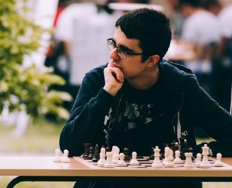
I met Mislav when he was a baby. Not an actual physical baby, mind you, but he was a baby to me and his sister, my very dear friend that I went to high school with. Think Dexter and Dee-Dee. We saw him as someone who'd outlive us both and never once questioned that belief until May 13th 2025, the day he unexpectedly passed. Maybe that's why the news is weighing so heavily on me even as I write this days later. Even then, he was a very sweet young man who had that spark of unbridled curiosity that is so uncommon in everyday people around us, a brilliance which is not obvious only to the malicious or the ignorant. That same brilliance is often isolating because the people who get us are few and far between, literally and physically. In the "real world", we learn to live a very lonesome life, but online...

Unbeknownst to most people, we have thriving social lives online in communities where we bond with others like us. We use alias names which become as real to us as our given names. This article is, in big part, for all of Mislav's friends who are soon going to get worried that he's no longer logging in. Approximately by the time this article gets indexed by Google, as our usual cope is that they're either working or on a vacation and lasts for about two weeks.

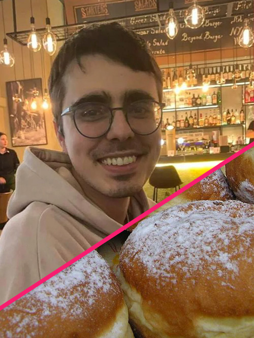
Cheeky as he was, hailing from Slavonia in Croatia, one of his public-facing and most persistent usernames online was Krofna and Krofnica. A bit of a tongue twister for Westerners, it means donut. But not the dog tier Amerikanski ones, the legit babushka stuff that was often made during the Kolinje season (traditional pig slaughter in November) and other fancy occasions. Generally they don't have a hole in the middle and were filled with pekmez (jam), which is clearly superior. If you imagined a torus, Mislav is definitely sighing at your uneducated peasant ass.

The search for Martin

In 2011, I met a crowd of people on StackOverflow who became my lifelong friends. We were quite polarizing and notorious because we created a lot of headaches for the maintainers of the website, but generally nice and helpful under all the nerd bluster. One of us was Martin, an elder of the group who one day went AWOL for a prolonged period of time. Naturally, due to his advanced age, we feared the worst. We tracked him down and contacted his wife, who told us he was at the pub. We were delighted to learn he was just doing what he does best... Drinking.

I regret you will not have a similar story to tell your friends about Mislav. But that event sparked discussion about the fact that all good things must end. One day all of us will go offline for the last time and it will be fairly difficult to validate what transpired. Hence, I am trying to do my friend Mislav one last favor, and let his friends know he did not abandon them of his own will.

About Mislav

Our krofnica.

Mislav was a 90s kid (albeit a little late to the party), just like most of us who knew him. From an early age, it was easy to see he wasn't a regular kid. Every mom likes to think their child is special, but Mislav genuinely was.

Unlike all of us, through his early life exposure to interactive entertainment, his natural inclination for figuring out how things work sparked an interest in computing, learning to program computers at an age when most of his peers were still struggling with registering on Facebook and installing sixteen viruses in a trench coat because they ran Kletva_Kralja_Zvonimira.exe thinking it would actually play a song. His sisters included.

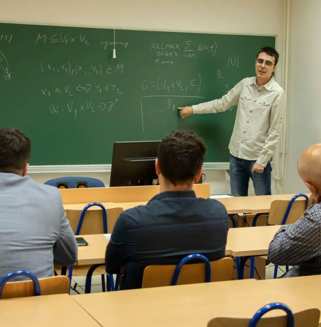
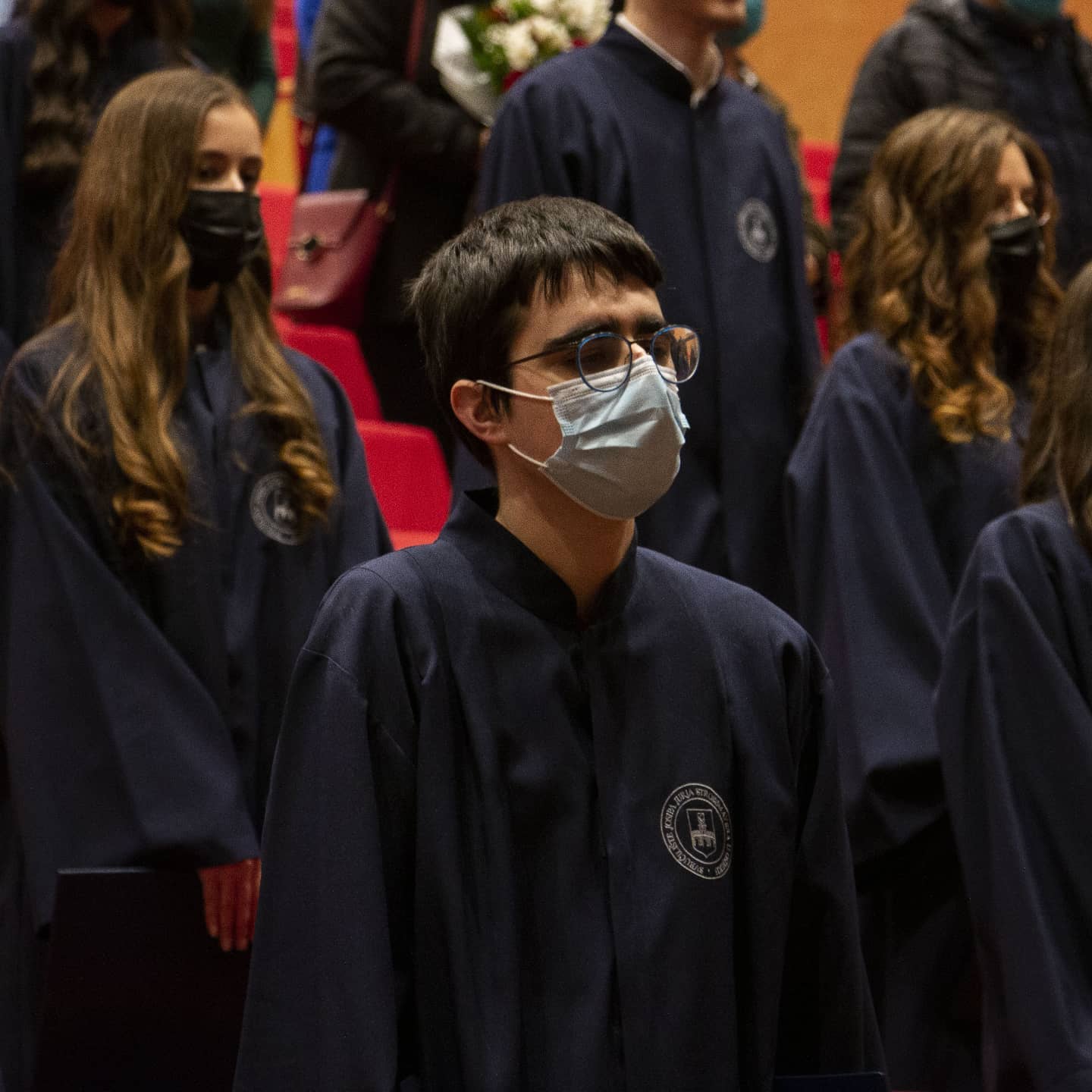
This interest naturally grew into a love of mathematics, in which he eventually successfully majored in, earning himself a position at Google. A kid from war-torn Slavonia, from humble beginnings and countless setbacks, the son of a war veteran, did all that.

As brilliant as he was, he was also very reserved. A man of few words socially and hard to gauge emotionally. It's not that he didn't feel things, just found it hard to express it, a trait we both share. Being vulnerable is hard for anyone, but especially so for brilliant people like Mislav. I got to know him in recent years a lot better, we joked a lot about politics in our favorite neighboring country, discussing math, physics, advances in many of the fields that are encompassed by computer science. I even got to learn a thing or two from him, the boy I drove home from the train station all those years back.

Mislav didn't want to go, but he couldn't stay. Remember him from time to time, I know I will. The universe exhibits periodic patterns on every scale, so I am certain we'll meet again. We won't remember any of this, but we'll recognize each other, I'm sure of it.

Addendum

His sister told me after the funeral that he appreciated and admired me. The feeling was mutual. The only thing that kept me from crying again were the sunglasses I kept on. I just wish I had made it more clear to him while he was around, but I think he knew.

Quantifying dipole radiation and deriving Rayleigh scattering coefficients
Domagoj Pandza on June 28th, 2022
Electrodynamics
Show in single article view
This is the updated version of the surprisingly popular article I wrote on the subject back in August of 2020. It incorporates all the feedback folks have given me thus far, hopefully improving overall didactic value. As usual, feel free to ask for further clarification on Discord.

One of the most cited papers on the subject of participating media rendering, "Display of The Earth taking into Account Atmospheric Scattering", published in 1993 by Tomoyuki Nishita et al. begins with an error in one of its equations. It raises the index of refraction $n$ to the power of $3$ instead of $2$ during the computation of the scattering coefficient $\beta$:

$$\beta \neq \frac{8\pi^3}{3N\lambda^4} \left(n^3 - 1 \right )^2 $$

Not a big deal, the author probably just did the classic mental oopsie of repeating $\pi^3$ on the neighbouring $n$ and seem to have used the proper equation they found in reference materials to calculate a set of coefficients which have been used religiously throughout every subsequent paper. However, and this is where it gets interesting, the coefficients in the original paper are inconsistently calculated and consequently technically wrong. Thanks to the game of academic broken telephone, all papers calling back on Nishita93 are technically wrong. I say technically because they're still perceptually plausible because you could miss by a mile and still get blue skies. Beyond having the ability to call foul on the color it detects, our brain is fairly easily fooled and will accept a wide margin of error in the variables the color depends upon. Truth be told, you don't need to do any physically accurate calculations, you can just eyeball them and it'll look just fine.

Still, if we're promising physically-based skies, we must tackle the issue of computing these coefficients as faithfully as possible (they are an approximation by definition). Even if you're just using predetermined equations, you still need to plug in consistently correct atmospheric state to yield the correct information at ground level. And this is somewhat tricky if you don't really understand it.

To demonstrate how this happened in Nishita93 and subsequent papers, take the Rayleigh scale height, it is "name-dropped" as $7994 \space \mathrm{m}$ with little qualification. That's the scale height if the assumed constant temperature of the atmosphere were around $0\textrm{°C}$. Targeting $0$ degrees is fine, a bit weird for a simulation, but those are the standard atmospheric conditions. "Normal" conditions ($20\textrm{°C}, 101.325\space\textrm{kPa}$) raise the scale height by more than $500$ meters. However, as long as you follow through with everything else, it's fine. After all, the sky is still blue during winter. But they didn't follow through. All papers citing Nishita use the same RGB wavelengths $(680, 550, 440)$ and the same scattering coefficients $(5.8, 13.5, 33.1)\times 10^{-6} \mathrm{m}^{-1}$. Trouble is, for a wavelength of $550$ nanometers at standard atmospheric pressure and $0\textrm{°C}$, you still get a scattering coefficient of approximately $12.1\times 10^{-6} \mathrm{m}^{-1}$ even if you round up the IOR of air to $1.0003$. The reference $13.5$ is achieved at $32\textrm{°C}$ where the particle number density is around $2.4\times 10^{25}$. To add more to this confusion, many of these papers also freely reference a number density of $2.55\times 10^{25}$ which happens around $14.6 \textrm{°C}$ without realizing the quantities are strongly interlinked. So, values used in subsequent integrals are, unwittingly, derived at three different temperatures.

What exactly is the atmosphere?

Back to basics.

Earth, like any other planet, boasts a gaseous mass bound to it by gravity that we collectively call the atmosphere. It's prominently heterogeneous, containing everything from life essentials such as nitrogen and oxygen to climate regulating molecules such as carbon dioxide via inert gases among which argon takes the cake at nearly 1%. For our purposes, it makes sense to separate it from localized phenomena such as aerosols which range from dust to clouds as well as the presence of free water vapor. Thus, we mostly speak of three primary constituents, namely, nitrogen (78%), oxygen (20%) and argon (0.9%).

For light emitted by the Sun to reach an observer on Earth, it needs to penetrate kilometers of atmosphere. This is somewhat eased by the fact that density reduces exponentially with altitude, and thus the amount of light scattered as you go towards the top. But, down here where we live, due to the way electric dipole radiation works, a significant amount of light you see is not directly from the Sun, it is n-ary re-radiation from induced dipoles in-scattering towards you.

Obviously, by looking up in the clear sky at day time, you conclude that this scattering is highly dependent on frequency and that it scatters blue light the most. This is made further evident when the Sun is towards the horizon and the path of the light is elongated to a point where all the blue light is out-scattered. The task for us is to quantify this and we begin by qualifying the assumptions we make about our atmosphere model.

The hydrostatic assumption

Dynamic bad, static good.

It should be clear to everyone that we can't hope to account for every particle in the atmosphere. We have to either rely on idealized models of the atmosphere or turn to statistics and probability theory, giving birth to statistical mechanics. Our ability to accurately predict the behavior of the atmosphere is thus extremely hampered, which you experience day in and day out with imprecise weather forecasts that don't really hold up on any interval other than a day or two.

For the purposes of rendering the atmosphere, we don't really need or want to model the atmosphere as a dynamic mess. The dynamics have no real discernible visual effect, it appears static (remember, we're ignoring water vapor, clouds, rain and other stuff right now). This enables us to assume that the atmosphere is a fluid at rest and there is no variations in pressure and density due to anything other than the column of air above the point being measured. There are no lateral forces to make our lives miserable. Oh, and we assume that the lapse rate of temperature is $0$, basically dealing with constant temperature throughout because we're lazy like that and it really doesn't matter.

Imagine a column of air of density $\rho$ and height $h$ reaching to the top of the atmosphere ("top" is discussed later), applying pressure on a horizontal area $A$ (volume is thus $V = Ah$). The pressure is then trivial:

$$P = \frac{F}{A} = \frac{mg}{A} = \frac{\rho V g}{A} = \frac{\rho Ahg}{A} = \rho g h$$

I'm pretty sure you worked this much out back in high school, it's one of those memorable, short equations. It enables you to calculate the ideal ground pressure, but what you really want to know is how it changes with as a function of altitude/height. What we're looking for is the rate of change of pressure $P$ with respect to height $h$, $dP/dh$. By using an infinitesimally small height, we can calculate the decrease in pressure as $-\rho g dh$, yes? In other words, we are one step away from having a canonical, ordinary, linear, homogeneous differential equation:

$$\frac{\partial P}{\partial h} = -\rho g \iff \frac{\partial P}{\partial h} + \rho g = 0$$

The step is relating $\rho$ and $P$ (they're interlinked) through the ideal gas law $PV = nRT$, specifically the form $PM = \rho RT$ ($n = m/M$) applicable here:

$$\frac{\partial P}{\partial h} = -\rho g \iff \frac{\partial P}{\partial h} + \frac{Mg}{RT}P = 0$$

Find the integrating factor, solve for $P$, couldn't be easier:

$$\Large{ P(h) = P_0 e^{-\frac{Mg}{RT}h} }$$

At this point, physicists like to add semantic spice/sugar to avoid lugging around the constants (and additionally confuse everyone new to the topic), $RT/Mg$ is declared to be the scale height and marked with $H$ which allows you to express it in a way that immediately gives away at which $h$ pressure (and density $\rho$ by direct extent) will be reduced by $e$:

$$\Large{ P(h) = P_0 e^{-\frac{h}{H}} \iff H = \frac{RT}{Mg} }$$

The star variable here is the molar mass $M$. For Rayleigh scattering, we use the molar mass of dry air which is $28.96 \space \mathrm{g/mol}$ which, at a pressure of one atmosphere ($101325 \space \mathrm{Pa}$) and $0\mathrm{°C}$ ($273.15 \space \mathrm{K}$), yields us a scale height between $7995$ and $7996$ meters provided you use the average Earth gravitational acceleration of $9.80665 \space \mathrm{ms^{-2}}$. If you use the more realistic temperature of $20\mathrm{°C}$, the scale height increases to a little less than $8600$ meters. Again, it doesn't matter, as long as you're consistent.

Electric dipole radiation

How does external radiation excite nitrogen et al. into radiating themselves?

Now we turn our attention to quantifying electric dipole radiation. As far as classical electrodynamics are concerned, light is nothing more than an electromagnetic wave propagating through space, mutually perpendicular and sustaining electric and magnetic fields oscillating in phase, amplitudes differing by a factor of $c$. While a dielectric such as a molecule of nitrogen might not have any net charge, its constituent matter is charged nonetheless. In a static electric field, the dielectric will "stretch" in the direction of the field and align with it due to the resulting torque. If you let the electric field oscillate, such as in the case of EM radiation, the direction and strength of the electric field will keep changing at a frequency associated with the radiation. While that happens, the forces on the dipole will never settle. In effect, you have a constantly jiggling dielectric and its constituent charges will be accelerating and decelerating.

And accelerating charges generate EM radiation. To easily picture this, it'll be squashing longitudinally with respect to its $\mathbf{E}$-aligned direction. While this is the way of thinking about it, considering accelerating charges and the radiation they generate is an unnecessary complication when we can just use the mathematically equivalent idea that the dipole charge separation $l$ is invariant and the amount of charge is oscillating.

Furthermore, it's a lot easier to deal with a perfect dipole instead of the mess that is, for example, a molecule of nitrogen. Such a setup merely has two opposite charges of equal, time-varying magnitude separated by a length $d$, changing harmonically. As you know from basic electrodynamics, a dipole moment is quantified as $\mathbf{p} = q\mathbf{l}$. Due to direct proportionality to the amount of charge and its separation, you can once more confirm that it is indeed mathematically sound to virtually oscillate the amount of charge $q$ instead of imagining the squashing action by modulating $\mathbf{l}$ and the ensuing mental overhead of considering accelerating charges explicitly. Henceforth, we can express a time-varying dipole moment as follows:

$$\Large{ \mathbf{p}(t) = q_0 \mathbf{l} \cos{\omega t} }$$

House rules

We assume that the scattering particle can be represented by a perfect dipole. We also assume that the particle in its induced dipole state is tremendously smaller than the wavelength of the light. We further posit that the light coming onto our stretchy bad boy is coming from the side and, as the electric and magnetic waves oscillate transversely to the direction of travel, we will conveniently align the electric field with the $z$ direction (yes, polarization). This means our dipole moment will also be aligned with the $z$ direction, which will simplify the math greatly as there will be zilch in $x$ and $y$ directions. This allows us to simplify further (well, mostly for me in 'TeX land):

$$\Large{ p(t) = q_0 l \cos{\omega t} \space \mathbf{\hat{k}} }$$

And off we go...

So, how do we recover the time-varying electric $\mathbf{E}$ and magnetic $\mathbf{B}$ fields from this? As usual in electrodynamics, we will be computing retarded potentials (don't giggle). These are "time-delayed" potential transforms where $t' = t - \Vert\mathbf{r}\Vert/c$. Outside of electrostatics, one needs both the scalar electric potential and the vector magnetic potential to recover the electric field and only the latter for the magnetic field. As, in the case of EM radiation, the electric and magnetic field magnitudes are related as $\mathbf{B}(...) = c\mathbf{E}(...)$ and perpendicular, we conclude that we only need to recover the vector magnetic potential which, again, from fundamental electrodynamics is calculated as:

$$ \mathbf{A}(\mathbf{r}, t) = \frac{1}{4\pi \epsilon_0 c^2} \int \frac{ \mathbf{I}(t)} {\Vert \mathbf{r}(l) \Vert} \space dl $$

As we have a changing charge situation, we inherently have a virtual current (you can imagine it going through the length $d$ of our interconnecting "wire" keeping the charges apart). We can easily express the current as the derivative of our oscillating charge subexpression from the original dipole moment equation:

$$ \mathbf{I}(t) = \frac{dq}{dt}\mathbf{\hat{k}} = -q_0\omega \sin{\omega t} \mathbf{\hat{k}} $$

And we can drop it into the mix:

$$ \mathbf{A}(\mathbf{r}, t) = \frac{1}{4\pi \epsilon_0 c^2} \int -\frac{ q_0\omega \sin{\omega ( t - \Vert\mathbf{r}\Vert/c )} } {\Vert \mathbf{r}(l) \Vert} \space dl \mathbf{\hat{k}} $$

Since we're very far away from the dipole moment, in the so-called radiation zone and given that the length $l$ is extremely small, we can get away by using a representative centered radius, distance to the observer from midway between the charges, call it simply $\mathbf{r}$. This demolishes the complexity of the integral as it completely removes any dependencies:

$$\begin{split} \mathbf{A}(\mathbf{r}, t) &= -\frac{q_0\omega }{4\pi \epsilon_0 c^2} \frac{\sin{\omega ( t - \Vert\mathbf{r}\Vert/c} )} {\Vert \mathbf{r} \Vert} \int dl \mathbf{\hat{k}} \\ & = -\frac{q_0 l \omega }{4\pi \epsilon_0 c^2} \frac{\sin{\omega ( t - \Vert\mathbf{r}\Vert/c )}}{\Vert \mathbf{r} \Vert} \mathbf{\hat{k}} \\ & = -\frac{p_0\omega }{4\pi \epsilon_0 c^2} \frac{\sin{\omega (t - \Vert\mathbf{r}\Vert/c)}}{\Vert \mathbf{r} \Vert} \mathbf{\hat{k}} \\ \end{split}$$

Cool? Cool. Now, since we have that pesky $\Vert\mathbf{r}\Vert$ in the $\sin$, it explodes any attempt to take the curl of $\mathbf{A}$ in 3D Cartesian coordinates. This requires us to transition to spherical polar coordinates and the associated bases. If you have somewhat of a background in vector calculus, you probably know that we have:

$$\begin{split} \mathbf{A}(\mathbf{r}, t) &= -\frac{p_0\omega }{4\pi \epsilon_0 c^2} \frac{\sin{\omega (t - \Vert\mathbf{r}\Vert/c)}}{\Vert \mathbf{r} \Vert} \mathbf{\hat{k}} \\ &= -\frac{p_0\omega }{4\pi \epsilon_0 c^2} \frac{\sin{\omega (t - r/c)}}{r} (cos\theta\hat{r} - sin\theta\hat{\theta}) \\ \end{split}$$

Need more information?

Let me know on Discord if you don't understand what follows. I might have to write an entire article on the subject of what a change of coordinates entails in the context of integration and differentation, but for now I am going to assume you're knowledgeable enough to follow.

The curl in spherical polar coordinates is expressed as follows:

$$\Large{\nabla \times \mathbf{A} = \frac{1}{r^2 \sin\theta} \begin{vmatrix} \mathbf{\hat{r}} & r\mathbf{\hat{\theta}} & r\sin\theta\mathbf{\hat{\phi}} \\ \frac{\partial}{\partial r} & \frac{\partial}{\partial \theta} & \frac{\partial}{\partial \phi} \\ A_r & rA_\theta & r\sin\theta A_\phi \\ \end{vmatrix}}$$

Notice that we don't have anything in the azimuthal direction, hence that's the only one that will end up being non-zero:

$$ \nabla \times \mathbf{A} = -\frac{p_0\omega^2 }{4\pi \epsilon_0 c^3r} \sin\theta \cos{\omega (t - r/c)}\mathbf{\hat{\phi}} = \mathbf{B} $$

Notice $\hat{\phi}$, this means we have a spherically propagating wave expanding in $\hat{r}$ with its magnetic field oscillating tangentially to the surface of the imaginary sphere. This means the electric field is oscillating in the $\hat{\theta}$ direction and merely has a different magnitude due to the $c$ factor:

$$ \mathbf{E} = -\frac{p_0\omega^2 }{4\pi \epsilon_0 c^2r} \sin\theta \cos{\omega (t - r/c)}\mathbf{\hat{\theta}} $$

If you're wondering what the minus sign is trying to tell us, it implies there's a phase difference to the incident radiation. As mentioned, power (irradiance) expands in the $\hat{r}$ direction and instantenously is valued as:

$$\begin{split} \mathbf{S} &= \epsilon_0 c^2 \mathbf{E} \times \mathbf{B} = \frac{1}{\epsilon_0 c^3} \left ( \frac{p_0\omega^2 }{4\pi r} \sin\theta \cos{\omega (t - r/c)} \right )^2 \mathbf{\hat{r}} \\ &= \frac{p_0^2\omega^4 }{16\pi^2\epsilon_0 c^3 r^2} \sin^2\theta \cos^2{\omega (t - r/c)} \mathbf{\hat{r}} \\ \end{split}$$

Instantenous irradiance is not particularly useful, so let's dump the $\cos$ by averaging over a full cycle, which comes down to reducing it by a factor of $2$:

$$ \mathbf{\overline{S}} = \frac{p_0^2\omega^4 }{32\pi^2\epsilon_0 c^3 r^2} \sin^2\theta \mathbf{\hat{r}} \iff \mu = \frac{1}{2\pi} \int_0^{2\pi}cos^2(x) \space dx = 1/2 $$

Given that irradiance is power per unit surface, by integrating over the surface of a sphere of radius $r$, we can accumulate the total emitted power:

$$\begin{split} P &= \int_0^{2\pi} \int_0^\pi \frac{p_0^2\omega^4 }{32\pi^2\epsilon_0 c^3 r^2} \sin^2(\theta) r^2 sin\theta d\theta d\phi \\ &= \frac{p_0^2\omega^4 }{32\pi^2\epsilon_0 c^3} \int_0^{2\pi} d\phi \int_0^\pi \sin^3(\theta) d\theta \\ &= \frac{p_0^2\omega^4 }{16\pi\epsilon_0 c^3} \left (\frac{3}{4}\int_0^\pi \sin(\theta) d\theta - \frac{1}{4}\int_0^\pi \sin(3\theta) d\theta \right ) \\ &= \frac{p_0^2\omega^4 }{16\pi\epsilon_0 c^3} \left (\frac{4}{3} \right ) = \frac{p_0^2\omega^4 }{12\pi\epsilon_0 c^3} = \frac{4\pi^3 p_0^2\nu^4 }{3\epsilon_0 c^3} = \frac{4\pi^3 p_0^2c }{3\epsilon_0 \lambda^4}\\ \end{split}$$

And with this, we have quantified the radiation of a perfect (or idealized) dipole moment without explicitly dealing with accelerating charges. Now, we will turn our attention to getting the canonical Rayleigh scattering coefficients by considering billions of these dipoles in a sample rectangular volume through which collimated sunlight propagates.

Finding the Rayleigh scattering coefficients

...in spirit of the original approximation

As we've discussed previously, the volume of air is composed of billions upon billions of scattering molecules, which can be considered to be spherical (before being exposed to an outside EM field). As the sky is our witness, the secondary radiation generated by the induced dipole moments showcases no fixed phase relations between the scattering entities which would dampen or complicate the propagation to the "far radiation zone" (us). Basically, the assumption is that the spacing between the particles is much larger than the wavelength of the incoming light. It isn't really, there are thermal/density fluctuations at play which eliminate phase relations. But, that's a book on its own. A book on scattering. Works for us, either way.

As density changes exponentially with altitude, the scattering coefficients will vary in a similar fashion. It is up to us, then, to determine the coefficients at ground level, the base values. We thus consider the passage of a beam of light through a volume of constant density. You can imagine us doing this measurement horizontally with negligible variations in altitude.

Provided a horizontal, collimated beam of sunlight, we can imagine it passing through a virtual aperature of area $A$. The power of the light going through that area can be recovered by integrating the Poynting vector across the virtual surface, it's $P_l = A\epsilon_0 c E_0^2/2$. To compute the amount of power scattered on the infinitesimally thin impact area, we will first consider a volume of particles aligned with said impact area. As light propagates through a volume, constituent light-scattering molecules will generate induced dipole moments when exposed to the incident light. As we know the average power of a single light-scattering molecule, on the wings of superposition, we can say that the total average power being shot out as secondary radiation will be the sum of all the individual dipole moment powers in that volume:

$$\Large{ P_d = NAd\frac{4\pi^3 p_0^2c }{3\epsilon_0 \lambda^4} }$$

We want the power scattered instantenously, on the "impact area". This much is easy, we just divide by $P_d$ by $d$ to get something we can ratio against the to the incident light power. The ratio $P_d/P_l$ is our $k$:

$$\Large{ k = N\frac{8\pi^3}{3\epsilon^2_0\lambda^4} \left (\frac{p_0}{E_0} \right )^2 = N\frac{8\pi^3}{3\epsilon^2_0\lambda^4} \alpha^2 }$$

Because we have made the assumption that all the scattering particles are small with respect to the wavelength of the incident light, we can speak of polarizability independently of frequency, which simplifies our life to the static case. Speaking of, we can use the wellknown relation between the dielectric constant $\epsilon$ and the polarizability $\alpha$ (feel free to translate it to index of refraction):

$$\alpha = \frac{3\epsilon_0}{N}\left (\frac{\epsilon - 1}{\epsilon + 2} \right ) \Rightarrow k = \frac{24\pi^3}{\lambda^4} \frac{1}{N}\left (\frac{\epsilon - 1}{\epsilon + 2} \right )^2 $$

Computing the scattering coefficient at altitude $h$ is then merely:

$$\Large{ k(h) = \frac{24\pi^3}{\lambda^4} \frac{1}{N}\left (\frac{\epsilon - 1}{\epsilon + 2} \right )^2 e^{-\frac{h}{H}}}$$

To recover the appropriate particle number density $N$ at absolute temperature $T$ and ground pressure $P_0$, make sure to use $PV = nRT$ and the fact that $N = nN_A$ where $N_A$ is the Avogadro constant. This is used in transmittance calculations in accordance with the Beer-Lambert law which you can derive similarly to the way we derived the formulation of exponential, hydrostatic pressure. You just kick over the vertical column and deal with radiative flux and its first order derivative, another homogeneous differential equation.

How does anisotropic texture filtering work?
Domagoj Pandza on May 25th, 2021
Computer Graphics
Show in single article view

For most people, anisotropic filtering is something you just flick on for instant gratification and then proceed to forget about it because the hardware does all the work automagically. Gamers crank it up to the maximum magic number of 16 in settings because it seemingly has no performance impact and programmers read that setting and just write it into the sampler's description. They know it makes things less blurry at oblique angles, but seldom how it does it.

I've been asked to make the problem more approachable numerous times; to provide a guided derivation which doesn't make people want to jump off a cliff. Specifically, the request was to skirt any mention of signal processing which is a tall order. I've been reluctant for many moons because postulating the problem clearly for people without a strong background is a non-trivial affair... But let's give it a shot.

Basics of texture mapping

Gotta be easy, right?

Early on, rasterizers only dealt with generating procedural detail across the surface of rasterized triangles. To add more realism, texture mapping was introduced. The idea was to encode surface details into a 2D array, an image, a texture that was stored in memory and accessed at runtime as needed. The contents of it can be anything you want, from material information to a drawing of Hello Kitty. One "wraps" it around the geometry by creating a mapping between it and the vertices. This is a non-trivial, challenging and even artistic process which involves creatively flattening a 3D mesh ("unwrapping") into a normalized 2D space with minimal seams, then storing those 2D coordinates of flattened vertices on the vertices as an attribute which we colloquially refer to as "UVs". Naturally, when accessing a texture, the normalized texture coordinates are first scaled by the dimensions of the texture being accessed. Depending on texture addressing mode, texture coordinates leaving the normalized range can be well-defined by allowing wrapping around (enabling tiling), edge clamping etc.

Vertices, and their attributes, get projected to the screen during rasterization. But before we can use these coordinates to actually access any texture, we need to interpolate them from the corners of the triangle being rasterized to the pixel we're currently processing. Correctly interpolating all the vertex attributes is of paramount importance, we have to account for perspective. Simply put, under the perspective transform, uniform steps in the image plane (iterating pixel by pixel of uniform width and height) do not necessarily map to uniform steps in the plane containing the triangle being interpolated. Triangle vertices in view space can have high differences in depth and, thus, we have to effectively interpolate linearly in the plane of the triangle. You can find my derivation here, but you can easily see the gist of it in the diagram below, the higher the tilt with respect to the image plane, the smaller the projection of the triangle. Naively interpolating on the projected triangle is thus wrong as $s \neq t$ .
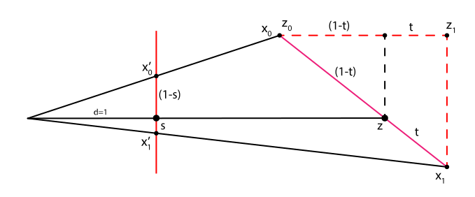
By finding the appropriate transform for said interpolation and fully simplifying it, we discover that the inverse of depth interpolates linearly in screen space. Knowing how to correctly interpolate $z$ allows us to solve for interpolated vertex attributes because the interpolation factor $t = (z - z_0) / (z_1 - z_0)$ is shared by any attribute $a$ being interpolated: $t = (a - a_0) / (a_1 - a_0)$. By equating the two, you can derive $a$. Some rearranging ahead, turns out vertex attributes divided by the associated vertex's depth interpolate linearly in screen space as $a/z = (1-t)a_0/z_0 + ta_1/z_1$, recovering the final value comes down to multiplying by the interpolated $z$. As texture coordinates are vertex attributes, we have our means for interpolating texture coordinates to pixel centers.

For those of you with a background in projective geometry with a solid grasp of homogeneous coordinates, none of this is news. Things of note to remember about projective mappings of any kind is that while they do preserve lines, they do not preserve parallel lines or equispaced points meaning that squares are mapped to generic quadrilaterals. Those are as useful as gasoline while trying to put out a fire at a nursing home.

So, what now? Do you just point sample the texture with the correctly interpolated texture coordinates? Hahah, no. That's your one-way ticket to Aliasville. To understand why not, consider your screen. A two-dimensional grid of square pixels (assume they're square for simplicity). Each pixel has a non-zero square area. Each, thus, must faithfully represent the area of a triangle projected to it. The projected triangle area may be covered by thousands of texels all competing for the attention of the poor single pixel, depending on the geometric relationship (distance, orientation) between the image plane and the plane containing the triangle. Huge area far away or tilted in view space projects to a tiny area. In other words, the partial derivatives of the texture coordinates wrt screen coordinates at the particular $(x,y)$ are huge.

Theoretically (and ideally), we can project the screen space pixel square into texture space where it morphs into a quadrilateral which covers the texels that desire to be considered. The goal is to iterate over all the texels covered by this quadrilateral (and not one more because ✨blur✨) and filter them into a single value to be used for the pixel being lit up. As you might imagine, this is computationally expensive to do at runtime. Any kind of direct convolution like this is, by definition.

In the 80s [notably Heckbert '86], a number of solutions performed the convolution offline, but with a twist. The unwieldy quadrilaterals are hard to handle mathematically, determining whether a texel is inside or out is non-trivial. Hence, Heckbert and those before him used to replace the projection with a local affine approximation, which approximates the unwieldy quadrilateral with a comparatively-tame parallelogram or an ellipse (if you modeled pixels as circles). This was still extremely expensive for realtime use, though, but it was doable. They used a weight LUT to actually figure out how each of the texels was weighted for the final filtered value to be computed. We can't afford the convolution at runtime, at all. We need to figure out a way to precompute this. At texture creation time, preferably.

Inventing "multum-in-parvo" maps

The multi-isotropic compromise

We can approximate a projection of the screen space pixel square (or circle) to a parallelogram (or ellipse) in texture space with a linear affine approximation, the details of which are the subject of next section. While that gives us the boundaries on the texels that require filtering, it's not particularly useful to us unless we can somehow prefilter the texture. It's not feasible to cover every possible "projected" parallelogram as you can see in the sample texture below:

Those are just a few examples and it is immediately obvious that no lookup structure can be devised here. What we could do is impose some restrictions on the filter shape, for example for it to be isotropic (same in every direction) and axis-aligned:

This kind of assumption makes creating the lookup structure a lot simpler, but it will not handle anisotropy well as a square naively approximating the parallelogram-shaped filter is going to capture texels outside of the filter shape, introducing overblurring in that direction. But if you think about it, we're not limited to picking just a single square. We can approximate a parallelogram-shaped filter by doing multiple square ones placed along the line of anisotropy (the "major axis" of the parallelogram):

To facilitate this isotropic prefilter structure, known as a mipmap, we create a hierarchy of textures where each level is quarter (or half if you're looking at dimensions individually) the resolution of the previous level and the data stored in it are the filtered values of all the $2 \times 2$ blocks of the previous level. This goes all the way to a level which is effectively a $1\times 1$ texture representing the filtered value of a $\textsf{w} \times \textsf{h}$ block of the texture. Since it's square and axis-aligned, you only need the center position (basically, the texture coordinates) and a single value to access the correct levels, the width of a square of texels we're filtering.

Reducing by $4$ on each level means it reduces by $2$ in each dimension. Given a width $w_f$ of square texels we're filtering (determined in the next section), we can take the $\log_2$ of $w_f$ to get a zero-based "index" into the levels. In quotes because it can have fractional parts, for example $\log(17) = 4.087$ meaning that we have to perform two bilinear samples on levels $4$ and $5$ and then use the fractional part $0.087$ to get the final filtered value, process called trilinear filtering. Final example, say $w_f$ turns out to be $2$, it means we want to access filtered $2 \times 2$ blocks. $\log_2(2)$ is $1$, meaning we want the first level where each texel represents filtered $2\times 2$ blocks of texels of the source texture (zeroth is the source texture) and so on. As we seldom want the actual blocks that were prefiltered and closer to those in-between, we perform bilinear filtering on the $4$ nearest texels each representing a filtered block of the source texture (size of block depends on level computed).

Rounding up texels

We're not going to hurt them, we just want to talk to them.

"Refactoring" update

I've incorporated some feedback over the past month for this article, hopefully increasing didactic value. I've also tried to use notation and shorthands that have engrained themselves over the decades, so mapping this article to reference final results can be easier while you're testing / getting a feel for everything. I'll try to design some diagrams when I feel better.

In the previous section, we found a way to prefilter our texture data and, from the diagrams, know that we need the line of anisotropy to determine the direction along which multiple isotropic mipmap samples are to be taken and the filter width $w_f$ from which we can compute the level(s) at which the mipmap will be sampled. According to the diagram, the line of anisotropy lies on the major axis of the ellipse drawn inside of our parallelogram of interest while the width $w_f$ can be derived from the distance from the extreme points on the ellipse along the minor axis. As you can clearly see, the ellipse can replace our parallelogram in the calculations and greatly simplify them as we only care about the extreme points on the ellipse (which are shared by the parallelogram). Thus, from now on, we'll use a circle instead of a square in all our calculations because ellipses intrinsically admit the notion of a major and minor axis.

As for the projection itself, it is reasonable to assume that we can approximate it with a locally-correct linear (affine) transform. To formulate such a transform, we need to determine how the texture coordinates change in the pixel's vicinity (the relationship between the two spaces). In other words, we're interested in computing the partial derivatives $\partial u/ \partial x$, $\partial u/ \partial y$, $\partial v/ \partial x$ and $\partial v/ \partial y$. Grouping these gives us two vectors indicating how $u$ and $v$ change in the XY plane around the point $(x,y)$, $\mathbf{dX}$ and $\mathbf{dY}$.

We don't actually compute partial derivatives proper on the GPU, pixel shaders instead execute in $2\times 2$ blocks which enables us to recover approximate screenspace partial derivatives via finite differencing (just subtracting), sufficient for practical applications dealing with discrete signals. By arranging our first-order partial derivative vectors as columns of a $2 \times 2$ matrix, we get a linear transform which approximately takes us to into texture space. This construct, when used more accurately, is known as the Jacobian (matrix):

$$\begin{split} \Large { \mathbf{J} = \begin{bmatrix} \frac{\partial u}{\partial x} & \frac{\partial v}{\partial x} \\ \frac{\partial u}{\partial y} & \frac{\partial v}{\partial y} \end{bmatrix}} \\ \end{split}$$

This linear transform, again, essentially approximates the reverse projection transform locally, we know how $(u,v)$ changes locally with respect to $(x,y)$. It is an approximation because we're assuming it'll be valid for more than just the point it was calculated on, ie the assumption of linearity is what is approximative.

So how do circles and ellipses work, again?

We've all dealt with circles at some point in our life, which are just a rotationally invariant kind of ellipse. The simplest formulation is usually $x^2 + y^2 = r^2$ which is trivial to understand. If you divide by $r^2$, you arrive at $(x/r)^2 + (y/r)^2 = 1$. You can see how the $r$ and $1$ on the right side constrict $x$ and $y$ isotropically from going beyond it. If you replace $r$ with $a$ and $b$, you can control the horizontal and vertical extent, effectively creating an ellipse centered on $(0,0)$ whose axes are aligned with the axes of the coordinate system:

$$\begin{split} \Large{\left(\frac{x}{a}\right)^2 + \left(\frac{y}{b}\right)^2 = 1} \\ \end{split}$$

This form is a bit bare-bones, but it gets the point across. The full, implicit equation for an arbitrary ellipse is:

$$\begin{split} ax^2 + bxy + cy^2 + dx + ey - f = 0 \\ \end{split}$$

$d$ and $e$ terms make the ellipse "leave" the origin and we're not particularly interested in them, so we drop them:

$$\begin{split} ax^2 + bxy + cy^2 - f = 0 \\ \end{split}$$

It can be converted into matrix form if you transform it a bit:

$$\begin{split} ax^2 + bxy + cy^2 &= f \\ ax^2 + \frac{b}{2}xy + \frac{b}{2}xy + cy^2 &= \\ x(ax + \frac{b}{2}y) + y(\frac{b}{2}x + cy) &= \\ \begin{bmatrix} x & y \end{bmatrix} \begin{bmatrix} a & b/2 \\ b/2 & c \end{bmatrix} \begin{bmatrix} x \\ y \end{bmatrix} &= \\ \end{split}$$

We have now shown that the following holds:

$$\begin{split} ax^2 + bxy + cy^2 = \mathbf{p}\mathbf{q}\mathbf{p}^\mathsf{t} = f \\ \end{split}$$

This is neat because we can apply transformations to our implicit ellipse parametrization as if it were any other primitive. However, there is a twist, we apply the inverse of whatever transform we have in mind. Intuition for this can be found in the way you translate something like a line to the right by actually moving the entire thing left on the $x$ term. Recall that $x$ and $y$ effectively go from $-\infty$ to $\infty$ and there's no transforming them. If we want to apply the transform $\mathbf{M}$ to facilitate $\mathbf{p'} = \mathbf{p}\mathbf{M}$, we plug in the inverse into a hypothetical ellipse $\mathbf{p'}\mathbf{Q'}\mathbf{p'}^\mathsf{T} = f'$ to yield:

$$\begin{split} \mathbf{p'}\mathbf{Q'}\mathbf{p'}^\mathsf{T} &= f'\\ \mathbf{pM^{-1}} \mathbf{Q'} \left(\mathbf{pM^{-1}}\right)^\mathsf{T} &= f'\\ \mathbf{pM^{-1}} \mathbf{Q'} \mathbf{M^{-1}}^\mathsf{T}\mathbf{p}^\mathsf{T} &= f' = f\\ \end{split}$$

We then have the transformed coefficient matrix specified as $\mathbf{Q} = \mathbf{M^{-1}} \mathbf{Q'} \mathbf{M^{-1}}^\mathsf{T}$. Also note that $f = f'$. Surely now you can see that one can start with a circle coefficient matrix (the identity matrix) and transform it into any ellipse. Further still, we can take a more generic, parametric formulation of the circle such as $\mathbf{p} = (\cos t, \sin t)$ and transform it arbitrarily then use $\mathbf{p}\mathbf{p}^{\textsf{T}} = \cos^2 t + \sin^2 t = 1$ to recover $\mathbf{Q}$ and $f$ of the implicit formulation.

Okay, now what?

What we're most interested in, though, is recovering the major and minor axis of the ellipse once we transform the parametric unit circle (representing our pixel) to the implicit ellipse using the finite difference relation clueing us in as to how texture space's $(u,v)$ changes locally with respect to screen space's $(x,y)$, our peasant-constructed Jacobian computed from $2\times 2$ blocks of pixels via finite differencing.

First things first, from the parametric unit circle to the implicit target ellipse. As mentioned, we have the Jacobian peasantly computed, so it comes down to merely transforming the points with it and recovering $\mathbf{Q}$ to get our $a, b, c, f$ coefficients:

$$\mathbf{p}\mathbf{p}^{\textsf{T}} = \cos^2 t + \sin^2 t = 1$$ $$\mathbf{p'M^{-1}} \mathbf{M^{-1}}^\mathsf{T}\mathbf{p'}^\mathsf{T} = 1 \iff \mathbf{p} = \mathbf{p'M^{-1}}$$ $$\mathbf{M^{-1}} \mathbf{M^{-1}}^\mathsf{T} = \frac{\begin{bmatrix} v_y & -v_x \\ -u_y & u_x \end{bmatrix} \begin{bmatrix} v_y & -u_y \\ -v_x & u_x \end{bmatrix}}{(u_xv_y - u_yv_x)^2} \iff M = \begin{bmatrix} u_x & v_x \\ u_y & v_y \end{bmatrix}$$

$f$ is in plain sight, it's just the denominator. The rest of them are a matrix multiply away, just map them to the $\mathbf{Q}$ entries:

$$\begin{split} a &= v_x^2 + v_y^2 \\ b &= -2(u_xv_x + u_yv_y) \\ c &= u_x^2 + u_y^2 \\ f &= (u_xv_y - u_yv_x)^2 \\ \end{split}$$

While we now have our circle "projected" to an ellipse in texture space, we need to find its major and minor axis that we'll be using for filtering (specifically, farthest points along those axes). The minor will be used to select the LOD of the mipmap and the major is our line of anisotropy we'll be sampling along at the LOD selected by the minor axis. Think back to our parametric circle prior to transform, it's a locus of points, yes? As we applied our linear transformation to it, the Jacobian, it elongated into an ellipse. There are four points on that ellipse which remained on the same two lines from the origin under the transform we performed, as if they were scaled by some value along a normalized direction which could replace the transform in that case. Yep, it's our major and minor direction "end points". This is a trivial (albeit tedious) eigenvalue and eigenvector determination problem.

Any ellipse centered around the origin can be viewed as the result of non-uniformly scaling and rotating a circle, meaning we can equate our Jacobian transform with the following:

$$\mathbf{M} = \mathbf{SR} = \begin{bmatrix} u_x & v_x \\ u_y & v_y \end{bmatrix} = \begin{bmatrix} a & 0 \\ 0 & b \end{bmatrix}\begin{bmatrix} \cos\theta & \sin\theta \\ -\sin\theta & \cos\theta \end{bmatrix}$$

The scaling is orthogonal while the rotation is orthonormal. As you know, the latter means rows are both mutually orthogonal and of unit length which makes its inverse equal to its transpose. Given that we define the transformed $\mathbf{Q}$ here as $\mathbf{M^{-1}}\mathbf{I}\mathbf{M^{-1}}^\mathsf{T}$, we have:

$$\mathbf{Q} = \mathbf{(SR)^{-1}}\mathbf{(SR)^{-1}}^\mathsf{T} = \mathbf{R}^{-1} \mathbf{S}^{-1} \mathbf{S^{-1}}^{\textsf{T}} \mathbf{R} = \mathbf{R}^{-1} \mathbf{S^{-2}} \mathbf{R}$$

Any well-behaved $n\times n$ matrix $\mathbf{A}$ encoding a linear transform will have $n$ eigenvalues and we should be able to find $n$ linearly independent eigenvectors. If you were to place all the eigenvectors as rows of a square matrix $\mathbf{E}$ and multiplied it with the associated matrix $\mathbf{A}$ the result would be a matrix where all the rows were multiplied with respective eigenvalues $\lambda_i$... As if you had built a diagonal square matrix containing eigenvalues $\mathbf{D}$ and multiplied it with $\mathbf{E}$ yielding $\mathbf{EA} = \mathbf{DE} \iff \mathbf{EAE^{-1}} = \mathbf{D}$. Going the "other way", we have $\mathbf{E^{-1}DE} = \mathbf{A}$. This leaves us with the following equivalence:

$$\mathbf{Q} = \mathbf{R}^{-1} \mathbf{S^{-2}} \mathbf{R} = \mathbf{E}^{-1} \mathbf{D} \mathbf{E}$$

Hence, $\mathbf{R} = \mathbf{E}$ and $\mathbf{S} = \mathbf{D}^{-1/2}$. Computing the eigenvalues for a generic $\mathbf{Q}$ amounts to:

$$\begin{bmatrix} x & y \end{bmatrix}\begin{bmatrix} (a - \lambda) & b/2 \\ b/2 & (c - \lambda) \end{bmatrix} = 0$$ $$(a - \lambda)(c - \lambda) - \frac{b^2}{4} = 0$$ $$\lambda^2 - (a+c)\lambda + \frac{4ac - b^2}{4} = 0$$ $$\lambda_{1/2} = \frac{a + c \pm \sqrt{(a+c)^2 - 4ac + b^2}}{2}$$ $$\lambda_{1/2} = \frac{a + c \pm \sqrt{(a-c)^2 + b^2}}{2}$$

It seems the square root and the $a \pm c$ terms will be following us around, so we might as well give them names. In the interest of keeping the result succinct, we can introduce the following substitutions $q = a + c, p = a - c, t = \sqrt{ p^2 + b^2}$. With $\mathbf{D}$, we easily resolve $\mathbf S$:

$$\mathbf{S} = \begin{bmatrix} \sqrt{\frac{2}{q + t}} & 0 \\ 0 & \sqrt{\frac{2}{q - t}} \end{bmatrix} \iff \mathbf{D} = \begin{bmatrix} \frac{q + t}{2} & 0 \\ 0 & \frac{q - t}{2} \end{bmatrix}$$

Going forward, remember that direction is our main concern, and as it aliases $\mathbf{R}$, we want them to be unit length and mutually orthogonal (a higher requirement than linear independence). Again, direction remains pristine. Thus, all shared magnitude-varying scalar factors will be dropped unceremoniously.

$$\begin{bmatrix} x & y \end{bmatrix}\begin{bmatrix} a & b/2 \\ b/2 & c \end{bmatrix} = \lambda_{1/2}\begin{bmatrix} x & y \end{bmatrix}$$ $$ax + \frac{b}{2}y = \lambda_{1/2}x \space \Rightarrow \space y = \frac{\pm t - p}{b}x$$ $$\frac{b}{2}x + cy = \lambda_{1/2}y \space \Rightarrow \space y = \frac{b}{\pm t + p}x$$

This nets us a pair of eigenvectors for each eigenvalue (remember the $\pm$):

$$\mathbf{e_{\lambda_{1/2}}} = \begin{bmatrix} b & \pm t - p \end{bmatrix}, \begin{bmatrix} \pm t + p & b \end{bmatrix}$$

Our goal is to normalize these vectors before moving forward, so let's do the first one of the first pair first... See what shakes out:

$$\begin{split} n_{\lambda_1,1} &= \sqrt{ (\pm t - p)^2 + b^2 } \\ &= \sqrt{ t^2 - 2tp + p^2 + b^2 } \\ &= \sqrt{ 2t^2 - 2tp } \\ &= \sqrt{2t}\sqrt{ t - p } \\ \end{split}$$

Similarly, you will find that $n_{\lambda_1,2} = \sqrt{2t}\sqrt{ t + p }$. Further, $n_{\lambda_2,i} = n_{\lambda_1,i}$ as the squaring action terminates the $\pm$ associated with $t$. But the biggest realization here is that $b$ doesn't contribute as a free term meaning that it has no bearing on the direction. We're then free to reuse the two distinct length calculations and recombine them into a single vector. Then, we can express the other vector as an implicit 90° rotation (as you know, swap the coordinates of the first one, negate one of them). This simplification will cost us some implicit sign information, but we can recover that from the sign of $b$. We have:

$$\mathbf{e_{\lambda_{1}}} = \begin{bmatrix} \sqrt{2t}\sqrt{ t + p } & \textsf{sgn}(b)\sqrt{2t}\sqrt{ t - p } \end{bmatrix}$$ $$\mathbf{e_{\lambda_{2}}} = \begin{bmatrix} -\textsf{sgn}(b)\sqrt{2t}\sqrt{ t - p } & \sqrt{2t}\sqrt{ t + p } \end{bmatrix}$$

As we isolated a scalar factor from all of them, we can drop it because it doesn't vary the direction:

$$\mathbf{e_{\lambda_{1}}} = \begin{bmatrix} \sqrt{ t + p } & \textsf{sgn}(b)\sqrt{ t - p } \end{bmatrix}$$ $$\mathbf{e_{\lambda_{2}}} = \begin{bmatrix} -\textsf{sgn}(b)\sqrt{ t - p } & \sqrt{ t + p } \end{bmatrix}$$

In this state, it becomes clear that the normalization factor of both is equivalent and it's $\sqrt{2t}$ which we will just prepend below. We set the two vectors as rows of $\mathbf{R}$ as it's equal to $\mathbf{E}$. Then we multiply it with $\mathbf{S}$. The rows of the resulting matrix represent the final directions for the major and minor axis.

$$\begin{split} \mathbf{M} = \mathbf{SR} &= \sqrt{\frac{1}{2t}} \begin{bmatrix} \sqrt{\frac{2}{q +t}} & 0 \\ 0 & \sqrt{\frac{2}{q - t}} \end{bmatrix} \begin{bmatrix} \sqrt{t + p} & \textsf{sgn}(b)\sqrt{t - p} \\ -\textsf{sgn}(b)\sqrt{t - p} & \sqrt{t + p} \end{bmatrix} \\ \end{split}$$

Therefore, our final expression for $\mathbf{M}$ is:

$$\begin{split} \large{ M = \begin{bmatrix} \sqrt{\frac{t+p}{t(q +t)}} & \textsf{sgn}(b)\sqrt{\frac{t-p}{t(q +t)}} \\ -\textsf{sgn}(b)\sqrt{\frac{t-p}{t(q - t)}} & \sqrt{\frac{t+p}{t(q - t)}} \end{bmatrix} }\\ \end{split}$$

From this we can calculate the farthest points of the ellipse along the normalized major and minor axis directions by factoring in $f$, to finalizing our boundary computation (if you can't figure out how $f$ works here, you're reading this article prematurely):

$$\mathbf{dX_{TS}} = \begin{bmatrix} \sqrt{f\frac{t+p}{t(q +t)}} & \textsf{sgn}(b)\sqrt{f\frac{t-p}{t(q +t)}} \end{bmatrix}$$ $$\mathbf{dY_{TS}} = \begin{bmatrix} -\textsf{sgn}(b)\sqrt{f\frac{t-p}{t(q - t)}} & \sqrt{f\frac{t+p}{t(q - t)}} \end{bmatrix}$$

These points can be interpreted as the transformed $\mathbf{dX}$ and $\mathbf{dY}$ vectors, hence the name. Doesn't really matter what you name them, though. Whichever of the two is longer can be thought of as defining the line of anisotropy. The shorter one, its length is more important. Specifically, you need to double it to get the width of the square filter we'll be using, the $\log_2$ of which nets us the mipmap level selection value. From there, $n$ trilinearly filtered samples are taken along the line of anisotropy (defined by the other vector) and filtered into a single value. $n$ is conservative, it is dynamically determined by the ratio of the anisotropy with a maximum defined by the user (and hardware). It tries to do it with least samples, unless the count of "least samples" is greater than the maximum anisotropy set by the user / programmer. At which point, it is clamped. The spacing of the samples is determined by the hardware, how much the axis-aligned squares end up overlapping affects weighing.

And in case you were wondering, yup, this is pretty much how Direct3D, OpenGL and Vulkan perform LOD and Line Of Anisotropy determination per specification. To properly get a feel for ellipses, I suggest you use these equations we derived on a graphing tool which are usually available online, my favorite is Desmos.