
In a previous article, we discussed how one can arrive at the van der Corput sequence, which is a low discrepancy sequence defined on the unit interval. While it is interesting on its own, generalizing it to higher dimensions is where it becomes useful in computer graphics applications. Applications where we often desire well distributed random samples that, for example, cover a domain uniformly for the purposes of estimating integrals. There is the standard approach of using pseudorandom number generators which have the unfortunate result of clumping samples together and poorly estimate integrals at low sample counts. As we've shown in the previous article, even though the van der Corput sequence is completely deterministic and predictable, it has the visual appearance of randomness (difficult to observe patterns) and has a very low upper bound on discrepancy meaning it is very near to being uniformly distributed.
Adding another dimension
The most trivial way to generalize the van der Corput sequence is to sample a separate van der Corput sequence for each axis. Obviously, they cannot be the same elements and they cannot be elements derived from the same sequence at some procedural offset as that creates a link between the two, an observable pattern. The only remaining thing to generalize then is the granularity at which the reflection around the radix point is performed, which in the vanilla case is derived from base \(2\). If we make it \(b\), the expression for our generalized van der Corput sequence becomes:
$$ \left( \sum_{k = 0}^{\log_b(i)+1}{d_k^b(i)b^{-k-1}} \right)_{i\in\mathbf{N}} $$
We desire to specify a sequence which constructs pairs or points, based on the generalized van der Corput sequence with an arbitrary base. We can specify one such sequence which maps from \(\mathbf{N}\) to \(\mathbf{R}^2\):
$$ \left( \left( \sum_{k = 0}^{\log_{b_0}(i)+1}{d_k^{b_0}(i)b_0^{-k-1}}, \sum_{k = 0}^{\log_{b_1}(i)+1}{d_k^{b_1}(i)b_1^{-k-1}} \right) \right)_{i,b_0,b_1\in\mathbf{N}} $$
Now, let's take it for a spin. We'll leave \(b_0\) at "native" \(2\) and set \(b_1\) to \(3\) because \(1\) is invalid. Here's \(32\) points with that configuration, we'll also prune the first element of the sequence, \((0,0)\) by means of a constant offset into the sequence, because it's not very useful:
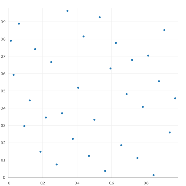
Taking the base pair \((2, 3)\) was the obvious and easiest first choice. Obviously, other choices work too with varying success. The larger the bases involved, the fewer digits are required to describe any given natural number. Let's take a look at what happens when we choose powers of \(2\) for the bases, by drawing 32 samples from a \((2, 4)\) sequence. You might guess this is a poor idea.
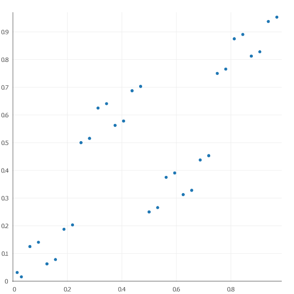
As you might imagine, choosing \(b_1 = 4\) is very much like using a constant offset into identical sequences, they become correlated and patterns emerge. Thus, we require the bases to be coprime, in other words, the only positive integer that divides both of them is \(1\). Anything else is equivalent to using the same base sequence with some offset. So, let's try a mutually prime pair, like \((4,3)\):
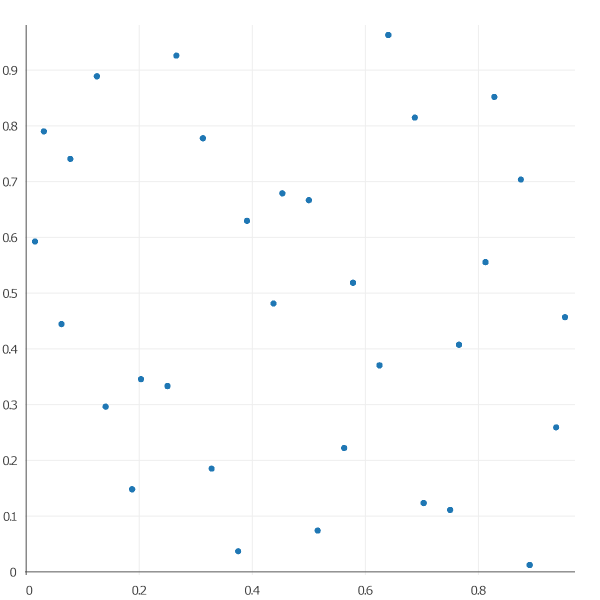
But even coprime bases will result in observable correlation once you get into the double digit bases such as \((16,13)\), as you can see below. Unlike the previous case, though, it is possible to avoid these issues but skipping a number of elements in the sequence depending on the bases used, as well as techniques involving scrambling or outright leaping.
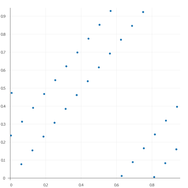
But really, keeping the bases coprime and low is the best option for most applications. The most commonly used bases are \((2,3)\), although I suspect most people use these due to appealing to authority, rather than understanding the issues involved. This type of sequence is called the Halton sequence, after the gentleman who proposed it in 1964.