
“Trivial to show” = I can’t be bothered/don’t remember how to redo this derivation
— Adam Solomon (@adamsolo) May 28, 2021
One of the most cited papers on the subject of participating media rendering, "Display of The Earth taking into Account Atmospheric Scattering", published in 1993 by Tomoyuki Nishita et al. begins with an error in one of its equations. It raises the index of refraction $n$ to the power of $3$ instead of $2$ during the computation of the scattering coefficient $\beta$:
$$\beta \neq \frac{8\pi^3}{3N\lambda^4} \left(n^3 - 1 \right )^2 $$
Not a big deal, the author probably just did the classic mental oopsie of repeating $\pi^3$ on the neighbouring $n$ and seem to have used the proper equation they found in reference materials to calculate a set of coefficients which have been used religiously throughout every subsequent paper. However, and this is where it gets interesting, the coefficients in the original paper are inconsistently calculated and consequently technically wrong. Thanks to the game of academic broken telephone, all papers calling back on Nishita93 are technically wrong. I say technically because they're still perceptually plausible because you could miss by a mile and still get blue skies. Beyond having the ability to call foul on the color it detects, our brain is fairly easily fooled and will accept a wide margin of error in the variables the color depends upon. Truth be told, you don't need to do any physically accurate calculations, you can just eyeball them and it'll look just fine.
Still, if we're promising physically-based skies, we must tackle the issue of computing these coefficients as faithfully as possible (they are an approximation by definition). Even if you're just using predetermined equations, you still need to plug in consistently correct atmospheric state to yield the correct information at ground level. And this is somewhat tricky if you don't really understand it.
To demonstrate how this happened in Nishita93 and subsequent papers, take the Rayleigh scale height, it is "name-dropped" as $7994 \space \mathrm{m}$ with little qualification. That's the scale height if the assumed constant temperature of the atmosphere were around $0\textrm{°C}$. Targeting $0$ degrees is fine, a bit weird for a simulation, but those are the standard atmospheric conditions. "Normal" conditions ($20\textrm{°C}, 101.325\space\textrm{kPa}$) raise the scale height by more than $500$ meters. However, as long as you follow through with everything else, it's fine. After all, the sky is still blue during winter. But they didn't follow through. All papers citing Nishita use the same RGB wavelengths $(680, 550, 440)$ and the same scattering coefficients $(5.8, 13.5, 33.1)\times 10^{-6} \mathrm{m}^{-1}$. Trouble is, for a wavelength of $550$ nanometers at standard atmospheric pressure and $0\textrm{°C}$, you still get a scattering coefficient of approximately $12.1\times 10^{-6} \mathrm{m}^{-1}$ even if you round up the IOR of air to $1.0003$. The reference $13.5$ is achieved at $32\textrm{°C}$ where the particle number density is around $2.4\times 10^{25}$. To add more to this confusion, many of these papers also freely reference a number density of $2.55\times 10^{25}$ which happens around $14.6 \textrm{°C}$ without realizing the quantities are strongly interlinked. So, values used in subsequent integrals are, unwittingly, derived at three different temperatures.
What exactly is the atmosphere?
Earth, like any other planet, boasts a gaseous mass bound to it by gravity that we collectively call the atmosphere. It's prominently heterogeneous, containing everything from life essentials such as nitrogen and oxygen to climate regulating molecules such as carbon dioxide via inert gases among which argon takes the cake at nearly 1%. For our purposes, it makes sense to separate it from localized phenomena such as aerosols which range from dust to clouds as well as the presence of free water vapor. Thus, we mostly speak of three primary constituents, namely, nitrogen (78%), oxygen (20%) and argon (0.9%).
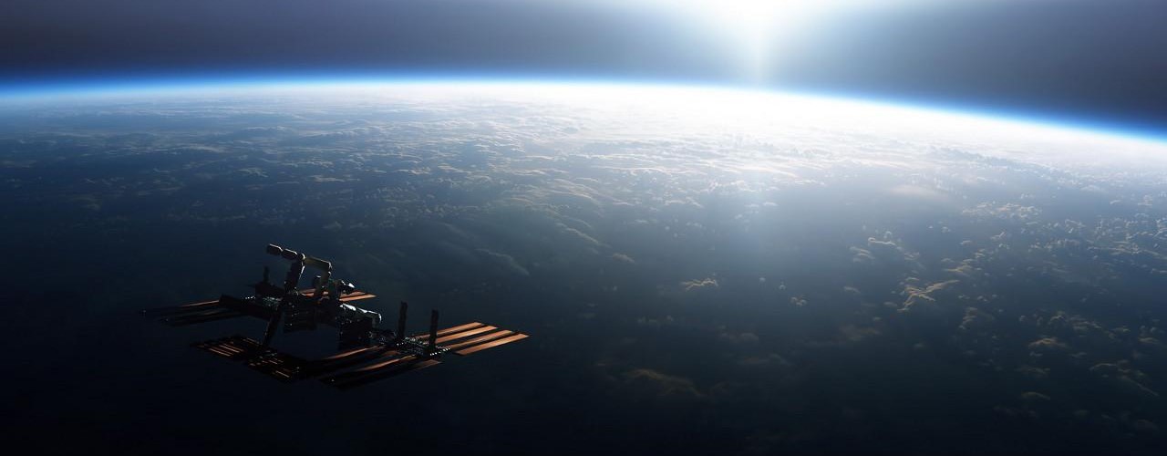
For light emitted by the Sun to reach an observer on Earth, it needs to penetrate kilometers of atmosphere. This is somewhat eased by the fact that density reduces exponentially with altitude, and thus the amount of light scattered as you go towards the top. But, down here where we live, due to the way electric dipole radiation works, a significant amount of light you see is not directly from the Sun, it is n-ary re-radiation from induced dipoles in-scattering towards you.
Obviously, by looking up in the clear sky at day time, you conclude that this scattering is highly dependent on frequency and that it scatters blue light the most. This is made further evident when the Sun is towards the horizon and the path of the light is elongated to a point where all the blue light is out-scattered. The task for us is to quantify this and we begin by qualifying the assumptions we make about our atmosphere model.
The hydrostatic assumption
It should be clear to everyone that we can't hope to account for every particle in the atmosphere. We have to either rely on idealized models of the atmosphere or turn to statistics and probability theory, giving birth to statistical mechanics. Our ability to accurately predict the behavior of the atmosphere is thus extremely hampered, which you experience day in and day out with imprecise weather forecasts that don't really hold up on any interval other than a day or two.
For the purposes of rendering the atmosphere, we don't really need or want to model the atmosphere as a dynamic mess. The dynamics have no real discernible visual effect, it appears static (remember, we're ignoring water vapor, clouds, rain and other stuff right now). This enables us to assume that the atmosphere is a fluid at rest and there is no variations in pressure and density due to anything other than the column of air above the point being measured. There are no lateral forces to make our lives miserable. Oh, and we assume that the lapse rate of temperature is $0$, basically dealing with constant temperature throughout because we're lazy like that and it really doesn't matter.
Imagine a column of air of density $\rho$ and height $h$ reaching to the top of the atmosphere ("top" is discussed later), applying pressure on a horizontal area $A$ (volume is thus $V = Ah$). The pressure is then trivial:
$$P = \frac{F}{A} = \frac{mg}{A} = \frac{\rho V g}{A} = \frac{\rho Ahg}{A} = \rho g h$$
I'm pretty sure you worked this much out back in high school, it's one of those memorable, short equations. It enables you to calculate the ideal ground pressure, but what you really want to know is how it changes with as a function of altitude/height. What we're looking for is the rate of change of pressure $P$ with respect to height $h$, $dP/dh$. By using an infinitesimally small height, we can calculate the decrease in pressure as $-\rho g dh$, yes? In other words, we are one step away from having a canonical, ordinary, linear, homogeneous differential equation:
$$\frac{\partial P}{\partial h} = -\rho g \iff \frac{\partial P}{\partial h} + \rho g = 0$$
The step is relating $\rho$ and $P$ (they're interlinked) through the ideal gas law $PV = nRT$, specifically the form $PM = \rho RT$ ($n = m/M$) applicable here:
$$\frac{\partial P}{\partial h} = -\rho g \iff \frac{\partial P}{\partial h} + \frac{Mg}{RT}P = 0$$
Find the integrating factor, solve for $P$, couldn't be easier:
$$\Large{ P(h) = P_0 e^{-\frac{Mg}{RT}h} }$$
At this point, physicists like to add semantic spice/sugar to avoid lugging around the constants (and additionally confuse everyone new to the topic), $RT/Mg$ is declared to be the scale height and marked with $H$ which allows you to express it in a way that immediately gives away at which $h$ pressure (and density $\rho$ by direct extent) will be reduced by $e$:
$$\Large{ P(h) = P_0 e^{-\frac{h}{H}} \iff H = \frac{RT}{Mg} }$$
The star variable here is the molar mass $M$. For Rayleigh scattering, we use the molar mass of dry air which is $28.96 \space \mathrm{g/mol}$ which, at a pressure of one atmosphere ($101325 \space \mathrm{Pa}$) and $0\mathrm{°C}$ ($273.15 \space \mathrm{K}$), yields us a scale height between $7995$ and $7996$ meters provided you use the average Earth gravitational acceleration of $9.80665 \space \mathrm{ms^{-2}}$. If you use the more realistic temperature of $20\mathrm{°C}$, the scale height increases to a little less than $8600$ meters. Again, it doesn't matter, as long as you're consistent.
Electric dipole radiation
Now we turn our attention to quantifying electric dipole radiation. As far as classical electrodynamics are concerned, light is nothing more than an electromagnetic wave propagating through space, mutually perpendicular and sustaining electric and magnetic fields oscillating in phase, amplitudes differing by a factor of $c$. While a dielectric such as a molecule of nitrogen might not have any net charge, its constituent matter is charged nonetheless. In a static electric field, the dielectric will "stretch" in the direction of the field and align with it due to the resulting torque. If you let the electric field oscillate, such as in the case of EM radiation, the direction and strength of the electric field will keep changing at a frequency associated with the radiation. While that happens, the forces on the dipole will never settle. In effect, you have a constantly jiggling dielectric and its constituent charges will be accelerating and decelerating.
And accelerating charges generate EM radiation. To easily picture this, it'll be squashing longitudinally with respect to its $\mathbf{E}$-aligned direction. While this is the way of thinking about it, considering accelerating charges and the radiation they generate is an unnecessary complication when we can just use the mathematically equivalent idea that the dipole charge separation $l$ is invariant and the amount of charge is oscillating.
Furthermore, it's a lot easier to deal with a perfect dipole instead of the mess that is, for example, a molecule of nitrogen. Such a setup merely has two opposite charges of equal, time-varying magnitude separated by a length $d$, changing harmonically. As you know from basic electrodynamics, a dipole moment is quantified as $\mathbf{p} = q\mathbf{l}$. Due to direct proportionality to the amount of charge and its separation, you can once more confirm that it is indeed mathematically sound to virtually oscillate the amount of charge $q$ instead of imagining the squashing action by modulating $\mathbf{l}$ and the ensuing mental overhead of considering accelerating charges explicitly. Henceforth, we can express a time-varying dipole moment as follows:
$$\Large{ \mathbf{p}(t) = q_0 \mathbf{l} \cos{\omega t} }$$
House rules
We assume that the scattering particle can be represented by a perfect dipole. We also assume that the particle in its induced dipole state is tremendously smaller than the wavelength of the light. We further posit that the light coming onto our stretchy bad boy is coming from the side and, as the electric and magnetic waves oscillate transversely to the direction of travel, we will conveniently align the electric field with the $z$ direction (yes, polarization). This means our dipole moment will also be aligned with the $z$ direction, which will simplify the math greatly as there will be zilch in $x$ and $y$ directions. This allows us to simplify further (well, mostly for me in 'TeX land):
$$\Large{ p(t) = q_0 l \cos{\omega t} \space \mathbf{\hat{k}} }$$
And off we go...
So, how do we recover the time-varying electric $\mathbf{E}$ and magnetic $\mathbf{B}$ fields from this? As usual in electrodynamics, we will be computing retarded potentials (don't giggle). These are "time-delayed" potential transforms where $t' = t - \Vert\mathbf{r}\Vert/c$. Outside of electrostatics, one needs both the scalar electric potential and the vector magnetic potential to recover the electric field and only the latter for the magnetic field. As, in the case of EM radiation, the electric and magnetic field magnitudes are related as $\mathbf{B}(...) = c\mathbf{E}(...)$ and perpendicular, we conclude that we only need to recover the vector magnetic potential which, again, from fundamental electrodynamics is calculated as:
$$ \mathbf{A}(\mathbf{r}, t) = \frac{1}{4\pi \epsilon_0 c^2} \int \frac{ \mathbf{I}(t)} {\Vert \mathbf{r}(l) \Vert} \space dl $$
As we have a changing charge situation, we inherently have a virtual current (you can imagine it going through the length $d$ of our interconnecting "wire" keeping the charges apart). We can easily express the current as the derivative of our oscillating charge subexpression from the original dipole moment equation:
$$ \mathbf{I}(t) = \frac{dq}{dt}\mathbf{\hat{k}} = -q_0\omega \sin{\omega t} \mathbf{\hat{k}} $$
And we can drop it into the mix:
$$ \mathbf{A}(\mathbf{r}, t) = \frac{1}{4\pi \epsilon_0 c^2} \int -\frac{ q_0\omega \sin{\omega ( t - \Vert\mathbf{r}\Vert/c )} } {\Vert \mathbf{r}(l) \Vert} \space dl \mathbf{\hat{k}} $$
Since we're very far away from the dipole moment, in the so-called radiation zone and given that the length $l$ is extremely small, we can get away by using a representative centered radius, distance to the observer from midway between the charges, call it simply $\mathbf{r}$. This demolishes the complexity of the integral as it completely removes any dependencies:
$$\begin{split} \mathbf{A}(\mathbf{r}, t) &= -\frac{q_0\omega }{4\pi \epsilon_0 c^2} \frac{\sin{\omega ( t - \Vert\mathbf{r}\Vert/c} )} {\Vert \mathbf{r} \Vert} \int dl \mathbf{\hat{k}} \\ & = -\frac{q_0 l \omega }{4\pi \epsilon_0 c^2} \frac{\sin{\omega ( t - \Vert\mathbf{r}\Vert/c )}}{\Vert \mathbf{r} \Vert} \mathbf{\hat{k}} \\ & = -\frac{p_0\omega }{4\pi \epsilon_0 c^2} \frac{\sin{\omega (t - \Vert\mathbf{r}\Vert/c)}}{\Vert \mathbf{r} \Vert} \mathbf{\hat{k}} \\ \end{split}$$
Cool? Cool. Now, since we have that pesky $\Vert\mathbf{r}\Vert$ in the $\sin$, it explodes any attempt to take the curl of $\mathbf{A}$ in 3D Cartesian coordinates. This requires us to transition to spherical polar coordinates and the associated bases. If you have somewhat of a background in vector calculus, you probably know that we have:
$$\begin{split} \mathbf{A}(\mathbf{r}, t) &= -\frac{p_0\omega }{4\pi \epsilon_0 c^2} \frac{\sin{\omega (t - \Vert\mathbf{r}\Vert/c)}}{\Vert \mathbf{r} \Vert} \mathbf{\hat{k}} \\ &= -\frac{p_0\omega }{4\pi \epsilon_0 c^2} \frac{\sin{\omega (t - r/c)}}{r} (cos\theta\hat{r} - sin\theta\hat{\theta}) \\ \end{split}$$
Need more information?
Let me know on Discord if you don't understand what follows. I might have to write an entire article on the subject of what a change of coordinates entails in the context of integration and differentation, but for now I am going to assume you're knowledgeable enough to follow.
The curl in spherical polar coordinates is expressed as follows:
$$\Large{\nabla \times \mathbf{A} = \frac{1}{r^2 \sin\theta} \begin{vmatrix} \mathbf{\hat{r}} & r\mathbf{\hat{\theta}} & r\sin\theta\mathbf{\hat{\phi}} \\ \frac{\partial}{\partial r} & \frac{\partial}{\partial \theta} & \frac{\partial}{\partial \phi} \\ A_r & rA_\theta & r\sin\theta A_\phi \\ \end{vmatrix}}$$
Notice that we don't have anything in the azimuthal direction, hence that's the only one that will end up being non-zero:
$$ \nabla \times \mathbf{A} = -\frac{p_0\omega^2 }{4\pi \epsilon_0 c^3r} \sin\theta \cos{\omega (t - r/c)}\mathbf{\hat{\phi}} = \mathbf{B} $$
Notice $\hat{\phi}$, this means we have a spherically propagating wave expanding in $\hat{r}$ with its magnetic field oscillating tangentially to the surface of the imaginary sphere. This means the electric field is oscillating in the $\hat{\theta}$ direction and merely has a different magnitude due to the $c$ factor:
$$ \mathbf{E} = -\frac{p_0\omega^2 }{4\pi \epsilon_0 c^2r} \sin\theta \cos{\omega (t - r/c)}\mathbf{\hat{\theta}} $$
If you're wondering what the minus sign is trying to tell us, it implies there's a phase difference to the incident radiation. As mentioned, power (irradiance) expands in the $\hat{r}$ direction and instantenously is valued as:
$$\begin{split} \mathbf{S} &= \epsilon_0 c^2 \mathbf{E} \times \mathbf{B} = \frac{1}{\epsilon_0 c^3} \left ( \frac{p_0\omega^2 }{4\pi r} \sin\theta \cos{\omega (t - r/c)} \right )^2 \mathbf{\hat{r}} \\ &= \frac{p_0^2\omega^4 }{16\pi^2\epsilon_0 c^3 r^2} \sin^2\theta \cos^2{\omega (t - r/c)} \mathbf{\hat{r}} \\ \end{split}$$
Instantenous irradiance is not particularly useful, so let's dump the $\cos$ by averaging over a full cycle, which comes down to reducing it by a factor of $2$:
$$ \mathbf{\overline{S}} = \frac{p_0^2\omega^4 }{32\pi^2\epsilon_0 c^3 r^2} \sin^2\theta \mathbf{\hat{r}} \iff \mu = \frac{1}{2\pi} \int_0^{2\pi}cos^2(x) \space dx = 1/2 $$
Given that irradiance is power per unit surface, by integrating over the surface of a sphere of radius $r$, we can accumulate the total emitted power:
$$\begin{split} P &= \int_0^{2\pi} \int_0^\pi \frac{p_0^2\omega^4 }{32\pi^2\epsilon_0 c^3 r^2} \sin^2(\theta) r^2 sin\theta d\theta d\phi \\ &= \frac{p_0^2\omega^4 }{32\pi^2\epsilon_0 c^3} \int_0^{2\pi} d\phi \int_0^\pi \sin^3(\theta) d\theta \\ &= \frac{p_0^2\omega^4 }{16\pi\epsilon_0 c^3} \left (\frac{3}{4}\int_0^\pi \sin(\theta) d\theta - \frac{1}{4}\int_0^\pi \sin(3\theta) d\theta \right ) \\ &= \frac{p_0^2\omega^4 }{16\pi\epsilon_0 c^3} \left (\frac{4}{3} \right ) = \frac{p_0^2\omega^4 }{12\pi\epsilon_0 c^3} = \frac{4\pi^3 p_0^2\nu^4 }{3\epsilon_0 c^3} = \frac{4\pi^3 p_0^2c }{3\epsilon_0 \lambda^4}\\ \end{split}$$
And with this, we have quantified the radiation of a perfect (or idealized) dipole moment without explicitly dealing with accelerating charges. Now, we will turn our attention to getting the canonical Rayleigh scattering coefficients by considering billions of these dipoles in a sample rectangular volume through which collimated sunlight propagates.
Finding the Rayleigh scattering coefficients
As we've discussed previously, the volume of air is composed of billions upon billions of scattering molecules, which can be considered to be spherical (before being exposed to an outside EM field). As the sky is our witness, the secondary radiation generated by the induced dipole moments showcases no fixed phase relations between the scattering entities which would dampen or complicate the propagation to the "far radiation zone" (us). Basically, the assumption is that the spacing between the particles is much larger than the wavelength of the incoming light. It isn't really, there are thermal/density fluctuations at play which eliminate phase relations. But, that's a book on its own. A book on scattering. Works for us, either way.
As density changes exponentially with altitude, the scattering coefficients will vary in a similar fashion. It is up to us, then, to determine the coefficients at ground level, the base values. We thus consider the passage of a beam of light through a volume of constant density. You can imagine us doing this measurement horizontally with negligible variations in altitude.
Provided a horizontal, collimated beam of sunlight, we can imagine it passing through a virtual aperature of area $A$. The power of the light going through that area can be recovered by integrating the Poynting vector across the virtual surface, it's $P_l = A\epsilon_0 c E_0^2/2$. To compute the amount of power scattered on the infinitesimally thin impact area, we will first consider a volume of particles aligned with said impact area. As light propagates through a volume, constituent light-scattering molecules will generate induced dipole moments when exposed to the incident light. As we know the average power of a single light-scattering molecule, on the wings of superposition, we can say that the total average power being shot out as secondary radiation will be the sum of all the individual dipole moment powers in that volume:
$$\Large{ P_d = NAd\frac{4\pi^3 p_0^2c }{3\epsilon_0 \lambda^4} }$$
We want the power scattered instantenously, on the "impact area". This much is easy, we just divide by $P_d$ by $d$ to get something we can ratio against the to the incident light power. The ratio $P_d/P_l$ is our $k$:
$$\Large{ k = N\frac{8\pi^3}{3\epsilon^2_0\lambda^4} \left (\frac{p_0}{E_0} \right )^2 = N\frac{8\pi^3}{3\epsilon^2_0\lambda^4} \alpha^2 }$$
Because we have made the assumption that all the scattering particles are small with respect to the wavelength of the incident light, we can speak of polarizability independently of frequency, which simplifies our life to the static case. Speaking of, we can use the wellknown relation between the dielectric constant $\epsilon$ and the polarizability $\alpha$ (feel free to translate it to index of refraction):
$$\alpha = \frac{3\epsilon_0}{N}\left (\frac{\epsilon - 1}{\epsilon + 2} \right ) \Rightarrow k = \frac{24\pi^3}{\lambda^4} \frac{1}{N}\left (\frac{\epsilon - 1}{\epsilon + 2} \right )^2 $$
Computing the scattering coefficient at altitude $h$ is then merely:
$$\Large{ k(h) = \frac{24\pi^3}{\lambda^4} \frac{1}{N}\left (\frac{\epsilon - 1}{\epsilon + 2} \right )^2 e^{-\frac{h}{H}}}$$
To recover the appropriate particle number density $N$ at absolute temperature $T$ and ground pressure $P_0$, make sure to use $PV = nRT$ and the fact that $N = nN_A$ where $N_A$ is the Avogadro constant. This is used in transmittance calculations in accordance with the Beer-Lambert law which you can derive similarly to the way we derived the formulation of exponential, hydrostatic pressure. You just kick over the vertical column and deal with radiative flux and its first order derivative, another homogeneous differential equation.